Normalization (two class meetings)

admin

Quick review of database anomalies

SLIDE 1 Suppose we begin with this table:

pID	name	team	teamPhone	pos1	pos2	pos3
1	Pessi	Argentina	54-11-1000-1000	str	for
2	Ricardo	Portugal	351-2-7777-7777	rm	dm
3	Neumann	Brazil	55-21-4040-2020	for	lb	rb
4	Baily	Wales	44-29-1876-1876	dm	st
5	Marioso	Argentina	54-11-1000-1000	sw	dm	st
6	Palé	Brazil	55-21-4040-2020	for

insert anomoly

SLIDE 2

pID	name	team	teamPhone	pos1	pos2	pos3
1	Pessi	Argentina	54-11-1000-1000	str	for
2	Ricardo	Portugal	351-2-7777-7777	rm	dm
3	Neumann	Brazil	55-21-4040-2020	for	lb	rb
4	Baily	Wales	44-29-1876-1876	dm	st
5	Marioso	Argentina	54-11-1000-1000	sw	dm	st
6	Palé	Brazil	55-21-4040-2020	for
∅	∅	Iceland	354-5-109-20	∅	∅	∅

We can’t add another team until we have a player on that team since the pID is the primary key.

update anomoly

SLIDE 3

pID	name	team	teamPhone	pos1	pos2	pos3
1	Pessi	Argentina	54-11-1000-1000	str	for
2	Ricardo	Portugal	351-2-7777-7777	rm	dm
3	Neumann	Brazil	55-21-4040-2020	for	lb	rb
4	Baily	Wales	44-29-1876-1876	dm	st
5	Marioso	Argentina	54-11-1000-1000	sw	dm	st
6	Palé	Brazil	55-21-4040-2020	for

If the Argentina team moves to a new facility in the suburbs, the teamPhone number will most likely change. This is made more difficult/error prone since there are multiple tuples that require update.

delete anomoly

SLIDE 4

pID	name	team	teamPhone	pos1	pos2	pos3
1	Pessi	Argentina	54-11-1000-1000	str	for
2	Ricardo	Portugal	351-2-7777-7777	rm	dm
3	Neumann	Brazil	55-21-4040-2020	for	lb	rb
4	Baily	Wales	44-29-1876-1876	dm	st
5	Marioso	Argentina	54-11-1000-1000	sw	dm	st
6	Palé	Brazil	55-21-4040-2020	for

If Ricardo retires from the Portugal team to become a coach for Sporting Clube de Portugal, we will need to delete his entry in this table. However, if we do that, we will lose the team and teamPhone information since he is the only player from Portugal in the table.

---

“Good” Relations

We’ve been talking about what makes a good database table.

• Few, if any, NULLs in typical use.
• Minimal keys.
• Little, if any, data redundancy.
• No anomalies.
• No lost information (we haven’t talked about this yet, but we will).

But when database designs get larger (and more realistic), or when someone else (like the customer) gave you a quick design “just to get you started”, identifying good vs. poor tables becomes less intuitive.

Today we begin talking about a generalized process called “normalization” which is a process for evaluating and correcting table structures to minimize data redundancies, thereby reducing the chance of data anomalies.

This normalization process identifies which attributes (columns) should be in which relations (tables) based on the their functional dependencies.

The normalization process involves transforming the set of relations into a series of Normal Forms (thus “normalization”).

SLIDE 5

• First normal form (1NF) and Second normal form 2NF aren’t talked about much - they are just steps on the way to higher normal forms.
• 3NF is typically enough for real use.
• 2NF is preferable to 1NF, and 3NF is preferable to 2NF and 1NF…

Academia studies higher forms (8NF?), but its unikely you will ever encounter them elsewhere.

There is another normal form between 3NF and 4NF called Boyce Codd NF, or BCNF which adds some desirable characteristics.

As is often the case in computer science, Normalization is not necessarily optimal for all situations.

• In general, the higher the NF the more joins you will need for typical queries.
  • This can use more run-time resources.
• If performance is a key attribute of the final system, then careful denormalization may be necessary.
  • The only real downside to denormalization is higher data redundancy.

As soon as you have ER models, you can begin.

• Goal is for all Relations to be well-formed.
  • Each Relation represents a distinct thing.
  • No Attribute will appear in more than one Relation.
• All attributes which are not part of the Primary Key are dependent on the Primary key.
• Every Relation is free of insertion, update, and deletion anomalies.
  • Working one relation at a time,
  • Determine the dependencies of a relation.
    • possibly breaking the relation up into multiple relations.

Before we begin learning about the details of the normalization process, we need to revisit Functional Dependencies (FD’s)[^DBCB] and learn how to reason about them.

[^DBCB]: Database Systems: The Complete Book; Garcia-Molina, et.al.

Functional Dependencies

Note: This section is derived from a superb lecture by Jennifer Widom of Stanford and the DBCB text.

The Normalization process depends upon the ideas of functional dependence. Let’s review:

Functional dependence: The value of one or more attributes determines the value of one or more other attributes.

• Determinant: Attribute whose value determines another
• Dependent: Attribute whose value is determined by another attribute

FD’s (as they are often abbreviated) are a generalized notion of keys, but they have other uses in databases beyond design:

• they enable more efficient data storage
• compression schemes can be used as a result
• they also enable some forms of query optimization

FD’s are based on knowledge of the real world of the entities you’re modeling.

All instances of a Relation must maintain the FD’s of that Relation … otherwise something is awry.

Formally

SLIDE 6

Write on board Let $R$ be a relation schema, and $\alpha$ and $\beta$ are sets of its attributes.

The functional dependency

$\alpha \rightarrow \beta$ holds on $R$ if and only if for any legal relations $r(R)$, whenever any two tuples $t_1$ and $t_2$ of $r$ agree on the attributes $\alpha$, they also agree on the attributes $\beta$. That is:

$$t_{1}[\alpha]=t_{2}[\alpha] \rightarrow t_{1}[\beta]=t_{2}[\beta]$$

An attribute $\beta$ is fully functionally dependent on the attribute $\alpha$ if each value of α determines exactly one value of $\beta$.

An attribute $\beta$ is fully functionally dependent on the composite attribute $\alpha$ if each value of α determines exactly one value of $\beta$ AND $\beta$ is not functionally dependent on any subset of the attributes in the composite key $\alpha$.

For example, in the Student table:

$$\text{STU\_NUM} \rightarrow \text{STU\_GPA}$$

However, if we say:

$$(\text{STU\_NUM, STU\_LNAME}) \rightarrow \text{STU\_GPA}$$

we find that STU_LNAME is not necessary to functionally determine STU_GPA. Thus, we see that STU_GPA is not fully functionally dependent on the composite attribute (STU_NUM, STU_LNAME).

---

DRAW ON BOARD

SLIDE 8

Let’s use our soccer tryouts example.

Player (pID, pName, pAddr, pHSID, pHSName, pHSCity, pRank, pPri)
Tryout(pID, cName, pos, decision)

Where $\text{pRank}$ in $\text{Player}$ is a percentage, as in “top 90%”.

Suppose tryout priority is determined by $\text{pRank}$:

pRank	priority
90-100	1
70-89	2
60-69	3

Here we can see that any two tuples (rows) in $\text{Player}$ that have the same $\text{pRank}$ will have the same priority.

Formally: if $s$ and $t$ are tuples of $R$, then

$$s.pRank = t.pRank \rightarrow s.pPri = t.pPri$$

Thus, this is a functional dependency for $R$ :

$$pRank \rightarrow pPri$$

In fact, we can generalize this to multiple attributes on either side:

$$s_{1}, s_{2}, ..., s_{n} \rightarrow t_{1}, t_{2}, ..., t_{n}$$

Note that a functional dependency need not include all of the attributes in the Relation.

What other FD’s can we see in this example?

$pID \rightarrow pName$ which makes sense in the real world.

$pID \rightarrow pAddress$ also makes sense, but only if you assume the student never moves!

Perhaps the same assumption for $pID \rightarrow pHSID$ if we assume only one $HS$

$pHSID \rightarrow pHSname, pHScity$ is another FD that seems intuitive.

Two attributes on the left works too $pHSname, pHScity \rightarrow pHSID$ since we assume no two $HS$’s in the same city have the same name.

As we said before $pID \rightarrow pRank$ and $pRank \rightarrow pPri$, so can we also say that $pID \rightarrow pPri$

SLIDE 9

The Tryout relation is tougher to find FD’s for.

If students can only tryout for one position at any given college, then we have $pID, CName \rightarrow Pos$

So, if we have a set of attributes $A$ in Relation $R$ that always determines all the other attributes $B$ then we can say that $A$ is a key for that Relation.

---

Types of FD’s

Trivial

Given the functional dependence $A \rightarrow B$, it is considered a Trivial FD if $B \subseteq A$.

For example, suppose we have $(NetID, LName) \rightarrow LName$.

Since $(LName) \subseteq (NetID, LName)$ , we have a Trivial FD.

Non-trivial

Given the functional dependence $A \rightarrow B$, it is considered a Non-Trivial FD if $B \not\subset A$.

That is, if B contains multiple attributes and at least one is not in $A$, it is a Non-Trivial FD:

$$B \not\subset A \text{, or equivalently, } A \cap B \neq \emptyset$$

For example, suppose we have

$$(NetID, LName) \rightarrow (LName, FName)$$

Since

$$(LName, FName) \not\subset (NetID, LName)$$

we have a non-Trivial FD.

But note that if two tuples agree in their $A$ values then they will also agree in their $B$ values, both inside $A$ and out.

Completely nontrivial

Given the functional dependence $A \rightarrow B$, it is considered a completely non-trivial FD if $A \cap B = \emptyset$.

For example, suppose we have

​ $(EmployeeID, Country) \rightarrow (Lname, FName, MI)$

Since

​ $(Lname, FName, MI) \not\subset (EmployeeID, Country)$

we have a non-Trivial FD. These are the most useful FD’s

Splitting Rule

This only works on the right side of an FD.

$$\bar{A} \rightarrow \bar{B}$$

means

$$\bar{A} \rightarrow B_1, B_2, ..., B_n$$

Thus, we can split the FD into $n$ FD’s:

$$\bar{A} \rightarrow B_1, \bar{A} \rightarrow B_2, ..., \bar{A} \rightarrow B_n$$

For example, suppose we have

$${HSID, COUNTRY} \rightarrow {HSCITY, HSNAME, HSENR}$$

We can split that into several FD’s:

$$\begin{align} {HSID, COUNTRY} &\rightarrow {HSCITY} \\ {HSID, COUNTRY} &\rightarrow {HSNAME} \\ {HSID, COUNTRY} &\rightarrow {HSENR} \end{align}$$

However, left side splitting doesn’t work. Suppose we have

$$\begin{align} pHSname, pHScity &\rightarrow pHSID \end{align}$$

we can’t split it to imply

$$\begin{align} pHSName &\rightarrow pHSID \end{align}$$

since there might be HS’s with the same name in different cities.

Combining Rule

This follows from the splitting rule:

$$A \rightarrow B_1, A \rightarrow B_2, ..., A \rightarrow B_n \quad \text{then} \quad A \rightarrow B_{1},...,B_{n}$$

Transitive Rule

$$if \quad A \rightarrow B \quad and \quad B \rightarrow C \quad then \quad A \rightarrow C$$

Full Functional Dependency

If $\bar{A}$ and $\bar{B}$ are each an attribute set of a relation, $\bar{B}$ is fully functional dependent on $\bar{A}$ if $\bar{B}$ is functionally dependent on $\bar{A}$ but not on any proper subset of $\bar{A}$.

Suppose we have different suppliers for a set of parts. Different suppliers may have different prices for the same part. Thus, we could not have a simple relation like

$$( \text{Part} ) \rightarrow ( \text{Price} )$$

Instead, we need a relation combining $Part$ and $Supplier$ as the determiner of the $Price$ :

$$( \text{Supplier},\text{Part} ) \rightarrow ( \text{Price} )$$

As you might guess, Partial Functional Dependency results when $\bar{B}$ is functionally dependent on $\bar{A}$ and $\bar{B}$ can be determined by any proper subset of $\bar{A}$.

$\bar{A}^+$ : Closure of attributes

Attribute closure of a subset of those attributes may be defined as the set of attributes which can be functionally determined from that original set.

To find the attribute closure of an attribute set:

1. Add elements of attribute set to the result set.
2. Recursively add elements to the result set which can be functionally determined from the elements of the result set.

Let’s try it with our soccer relations ON THE BOARD WITH STUDENTS

$$\begin{align} \text{Player} &\text{(pID, pName, pAddr, pHSID, pHSName, pHSCity, pRank, pPri)} \\ \text{Tryout} &\text{(pID, cName, pos, decision)} \end{align}$$

We have these functional dependencies:

$$\begin{align} \text{pID} &\rightarrow \text{pName, pAddr, pRank} \\ \text{pRank} &\rightarrow \text{pPri} \\ \text{pHSID} &\rightarrow \text{pHSname, pHScity} \end{align}$$

We want to find the closure of the attribute set $\lbrace pID,pHSID \rbrace^+$. That is, we want to find all of the attributes that are functionally determined by those in this initial set. \begin{align} &\lbrace pID, pHSID \rbrace \\ &\lbrace pID, pHSID, pName, pAddr, pRank \rbrace \\ &\lbrace pID, pHSID, pName, pAddr, pRank, pPri \rbrace \\ &\lbrace pID, pHSID, pName, pAddr, pRank, pPri, pHSname, pHScity \rbrace \end{align}

and we’re done now because this is all of the attributes in the relation!

Thus, if all the attributes in a relation can be functionally determined by the attributes $\lbrace pID, pHSID \rbrace$, that is the definition of a key for that relation!

Thus, we can determine whether some attribute set $\bar{A}$ is a key by computing ${\bar{A}^+}$ and if that produces all attributes in the relation then the original set is a key.

Finding all possible keys for a set of FD’s

Slide 10

We can also find all the possible keys if we’re given the relation and a set of FD’s by considering every subset of the attributes and then running the algorithm to see if that subset functionally determines all the attributes!

This would likely be really slow if we have a lot of attributes. However, there is a simple optimization: first try all the single attributes one at a time to determine whether any of them is a key. If you find a key then, as we saw earlier, every combination of attributes that contain that attribute is also a key. This notably reduces the computation.

Activity

Slide 11

---

— End of first day —

---

Normalization

A process for minimizing data redundancies and data anomalies

Involves redistributing attributes between tables, creation of new tables and relations.

The interim steps of normalization are called normal forms or NF. Lowest is 1st NF, and we will look at 2nd NF, 3rd NF, and one more called BCNF that’s just a little bit better than 3rd NF. These are generally written as $\text{1NF, 2NF, 3NF, ...}$

The higher numbered forms are better, in general, but denormalization may be appropriate for performance / efficiency reasons.

Do normalization as soon as you have an accepted ERD.

Changes resulting from normalization need to be reflected back in your ERD for documentation!

Restating our goals: All Relations will be well-formed

• Each relation represents a distinct thing
• No non-key attribute will appear in more than one relation
• All attributes which are not part of the Primary Key are dependent on the Primary key
• Every relation is free of insertion, update, and deletion anomalies.

NF Summary SLIDE 13

Kriz Wenzel summarrized the first three NF’s this way:

First Normal Form – The information is stored in a relational table and each column contains atomic values, and there are not repeating groups of columns.
Second Normal Form – The table is in first normal form and all the columns depend on the table’s primary key.
Third Normal Form – the table is in second normal form and all of its columns are not transitively dependent on the primary key

1NF

Steps:

1. Eliminate the repeating groups
2. Identify the PK
3. Identify all FD’s
4. Verify all attributes depend on PK

Here is an example (from the text) that has all sorts of issues. Slide 14

Explain Repeating groups (empty entries are a hint, see EMP_NUM)

In other words (Jukic):

A table is in 1NF if each row is unique and no column in any row contains multiple values from the column’s domain.

Generally all the tables we’ve used are in 1NF … but customer’s designs may not be.

Here’s the table after we convert it to 1NF:
Slide 15

Dependency diagrams

Shows all the dependencies within a Relation

It makes it easier to see how they all fit together, helps keep track of them

Develop the Dependency diagram on the board.

Here’s the 1NF Dependency diagram:
Slide 16

Note there are still potential problems:

• Alice submits a timesheet with multiple entries
  • Each one has EMP_NAME, JOB_CLASS, CHG_HOUR
  • Repetitious and error prone
• When someone is added to a project
  • PROJ_ID, PROJ_NAME, EMP_NUM, EMP_NAME, JOB_CLASS, and CHG_HOUR are entered each time – TYPOS!
  • EMP_NUM should be enough to rep the EMP_NAME, JOB_CLASS, and CHG_HOUR
• Others?

Partial Functional Dependencies

Suppose you have α → β and α is actually a compound of two (or more) attributes, α₁ and α₂.

If β is actually functionally determined by only one of them, say α₁ , then this is a partial dependency.

This is what we saw in the 1NF Dependency Diagram in Slide 16.

Transitive dependencies

If neither α nor β are part of the primary key, then α → β is a Transitive dependency.

Conversion to 2NF

2NF means:

• 1NF, and
• no partial dependencies

Steps

1. Make new tables to eliminate partial dependencies
2. Reassign corresponding dependent attributes

Kris’ way to think about it is to go through each non-primary-key attribute and ask yourself

“Does this column serve to describe what the primary key identifies?”
If not, then move it out.

1. Create a new table for each component of the PK that is a determinant in a partial dependency, using that component as the new table’s Primary Key. Leave a copy behind as a Foreign Key.
2. Update the tables on the board to identify the partial dependencies and then make new relations by removing the dependent attributes into new relations with their determinant as primary key.

This adds PROJECT, EMPLOYEE, and ASSIGNMENT

We created ASSIGNMENT because the HOURS an employee worked depends on the EMP_ID and the PROJ_NUM. Yes, it’s a compound Primary Key.

Here’s the new dependency diagram for 2NF Slide 17

Much better, but we still have a transitive dependency which can be problematic.

• EMP_NUM determines JOB_CLASS and CHG_HOUR, JOB_CLASS also determines CHG_HOUR
  • If there is a CHG_HOUR change for a JOB_CLASS, you will have to be very careful to ensure that all instances of EMP_NUM’s with that JOB_CLASS have their CHG_HOUR updated the same way.

Conversion to 3NF

3NF means:

• 2NF, and
• no transitive dependencies

Steps:

1. Make new relations to eliminate transitive dependencies
2. Reassign corresponding dependent attributes

Identify the transitive dependency and make a new relation by copying the determinant into a new relation as primary key and moving its dependent attributes with it.

Leave the determinant in the original table to act as a foreign key.

Slide 19

And that’s 3rd NF !

Other improvements

• Review PK definitions
  • a new EMPLOYEE entry requires a entry of a JOB_CLASS. This is a string, which can be typoed.
• Check naming conventions
  • rename attributes to match their table, like CHG_HOUR becomes JOB_CHG_HOUR
  • strive for consistency
• Review Attributes for atomicity (cannot/shouldn’t be further subdivided)
  • EMP_NAME certainly has multiple parts - fix it!
• Missing attributes and relations?
  • Lots of real-world stuff would need to be added to EMPLOYEE table.
  • Some employees are managers of projects - how would we show that?
  • Customers don’t always think of these.
• Evaluate using derived attributes or storing them?
  • time vs. space, as usual
• Ensure proper granularity of PK’s
  • Can you access the data at the desired level of detail?
  • Address as a whole, or do you need access to zip?
• Be careful about history, backwards compatibility with old tables and other applications
  • may need “bridge relations”.

Show the final DB:
Slide 20 and Slide 21

In summary:

data depends on the key [1NF], the whole key [2NF] and nothing but the key [3NF].

• Author unknown (to me at least)

---

BCNF

SLIDE 22

First a review of the types of keys:

• Composite Key
  a key composed of > 1 attributes
• Superkey
  a key that can uniquely identify any row in the relation
• Candidate key
  a minimal Superkey – one that has no unnecessary attributes
• Primary key
  a Candidate key that was selected as the Primary and can never be NULL

Boyce-Codd Normal Form is a special case of 3NF, some call it 3.5NF

It goes a little beyond 3NF because it requires the removal of all redundancy based on FD’s.

A Relation is in Boyce-Codd Normal Form (BCNF) when

1. it is in 3NF, and
2. the left side of every non-trivial FD (the determinant) of the Relation is a Superkey.

If a relation has only one Candidate key, 3NF and BCNF are equivalent for that relation.
Thus, BCNF can only be violated if there is more than one candidate key

• Formal definition:
  • We say a relation $R$ is in BCNF if whenever $X \rightarrow Y$ is a nontrivial FD that holds in $R$, then $X$ is a superkey.
  • Remember: nontrivial means $Y$ is not contained in $X$.

BCNF and non-BCNF Examples: SLIDE 23,24

Example 1 from Garcia-Molina

$$Drinkers(\underline{name}, addr, \underline{beersLiked}, brewer, favBeer)$$

Functional Dependencies (FD’s):

$$\begin{align} name&\rightarrow addr, favBeer \\ beersLiked&\rightarrow brewer) \end{align}$$

• In each FD, the left side is not a superkey.
• Thus, either FD shows the Relation is not in BCNF

Example 2 from Garcia-Molina

$$Beers(\underline{name}, manf, manfaddr)$$

FD’s:

$$\begin{align} name&\rightarrow manf \\ manf&\rightarrow manfaddr \end{align}$$

Thus, $name\rightarrow manf$ does not violate BCNF, but $manf\rightarrow manfaddr$ does.

Converting to BCNF

• Start with the offending FD: $X \rightarrow Y$ for the relation $R$
• Compute $X^+$ (which isn’t all attributes, since that would make $X$ a superkey)
• Replace $R$ with new relations with these schemas:

$$\begin{align} R_1 &= X^+ \text{and} \\ R_2 &= R-(X^+ - X) \end{align}$$

Continuing the G-M example:

$$Drinkers(\underline{name}, addr, \underline{beersLiked}, brewer, favBeer)$$

• Choose FD that violates BCNF: $name\rightarrow addr$ using splitting rule
• Find closure of ${name}^+ = {name, addr, favBeer}$
• Decomposed relations:

$$\begin{align} Drinkers1&(\underline{name}, addr, favBeer) \\ Drinkers2&(\underline{name}, \underline{beersLiked}, manf) \end{align}$$

• Are we done? No, we do it again until no BCNF violations

  1. For $Drinkers1$ the relevant FDs are
  $$\begin{align} name&\rightarrow addr \\ name&\rightarrow favBeer \end{align}$$

  Thus, ${name}$ is the only key and $Drinkers1$ is in BCNF.

1. For $Drinkers2$ the only FD is

$$\begin{align} beersLiked&\rightarrow manf \end{align}$$

and the only key is ${name, beersLiked}$, which is a violation of BCNF, so we do it again

1. ${beersLiked}^+ = {beersLiked, manf}$, so we decompose $Drinkers2$ into:

$$\begin{align} Drinkers3&(\underline{beersLiked}, manf) \\ Drinkers4&(\underline{name}, \underline{beersLiked}) \end{align}$$

The final result of the decomposition of Drinkers is:

$$\begin{align} Drinkers1&(\underline{name}, addr, favBeer) \\ Drinkers3&(\underline{beersLiked}, manf) \\ Drinkers4&(\underline{name}, \underline{beersLiked)} \end{align}$$

Where

$$\begin{align} Drinkers1 &\text{ tells us about drinkers,} \\ Drinkers3 &\text{ tells us about beers, and} \\ Drinkers4 &\text{ tells us the relationship between drinkers and the beers they like.} \end{align}$$

Another example (from Silberschatz)

Suppose we are given:

$$instrDept (\underline{ID}, name, salary, \underline{deptName}, building, budget)$$

with FD:

$$deptName\rightarrow building, budget$$

But $deptName$ is not a superkey of $instrDept$ :

$${deptName}^+ = {deptName, building, budget}$$

so we decompose into

$$\begin{align} instrDept_1 &= (deptName, building, budget) \\ instrDept_2 &= (ID, name, salary, deptName) \end{align}$$

---

So what does this buy us?

There are two important properties of any decomposition:

1. Lossless Join : it should be possible to project the original relations onto the decomposed schema, and then reconstruct the original.
2. Dependency Preservation : it should be possible to check in the projected relations whether all the given FD’s are satisfied.

Not all decompositions are good. Here’s an example from Silberschatz:

Decompose

$$employee(ID, name, street, city, salary)$$

into

$$\begin{align} employee1&(ID, name) \\ employee2&(name, street, city, zip) \end{align}$$

Can we reconstruct the original relation? NO!

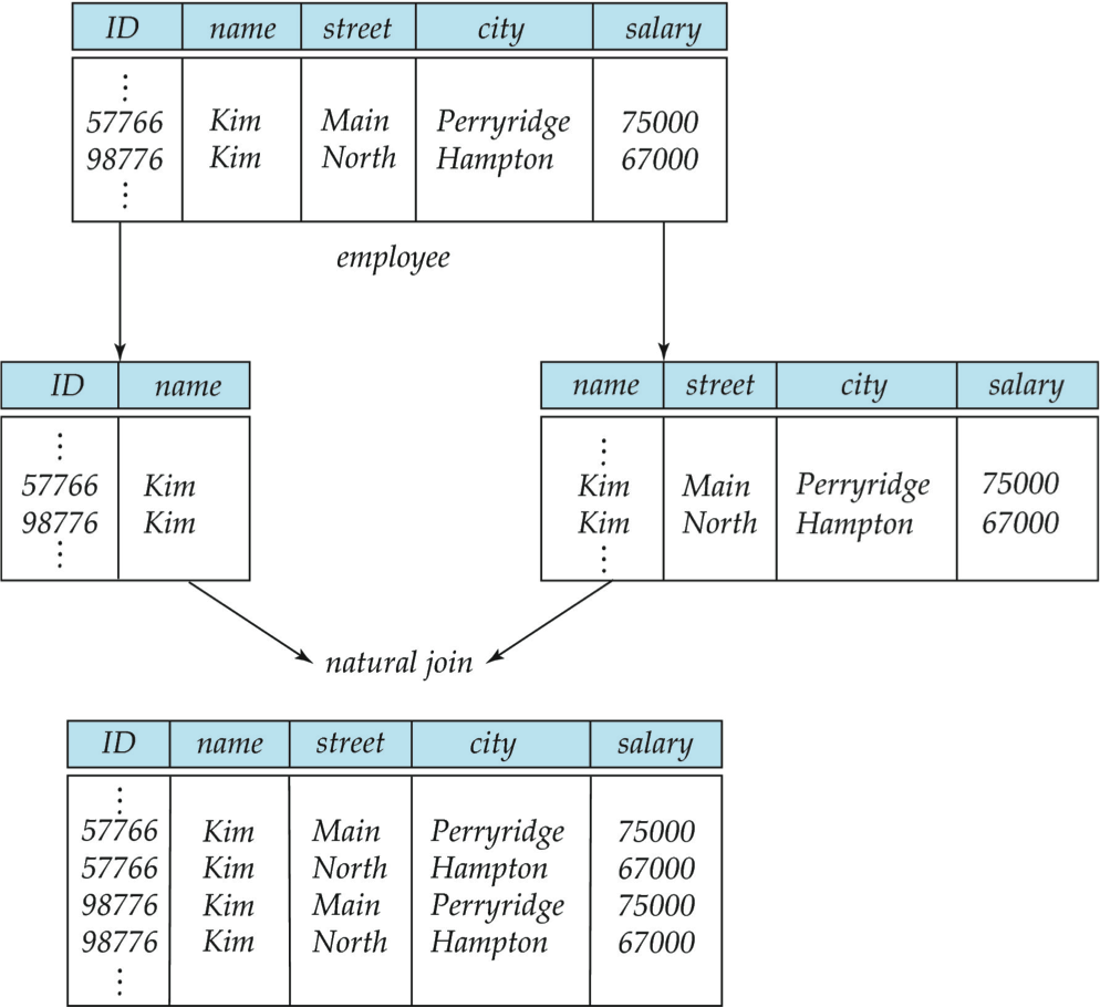
Not good!

A decomposition that is not lossless is called Lossy.

The 3NF conversion process ensures no losses.

Denormalization

Our design goals have been

• Creation of normalized relations
• Processing requirements and speed

Motivations were due to defects in unnormalized tables

• Data updates are less efficient because tables are larger
• Indexing is more cumbersome
• No simple strategies for creating virtual tables known as views (we’ll see this later)

However, the number of database tables expands when tables are decomposed to conform to increasing normalization requirements.

This results in having to join a larger number of tables to use the DB

• Takes additional input/output (I/O) operations and processing logic
• Reduces system speed

Common examples of denormalization:

• derivable data

  • storing both MILES_FLOWN and AWARD_LEVEL in a frequent flyer DB since AWARD_LEVEL is derivable from MILES_FLOWN.
  • However, it avoids extra joins, enables auditing since AWARD_LEVEL can be verified by looking at MILES_FLOWN.

• Preaggregated data

  • Storing GPA when it could be calculated from the ENROLLED and COURSE tables.
  • This also avoids extra joins and the GPA is recomputed everytime a grade is entered or updated.

Review of Data Modeling

SLIDE 25-28