On-Road Vehicle Detection in Static Images
Zhipeng Hu
Introduction
As vehicles improved with technological advancements, faster speeds were attained and more serious accidents were caused. Vehicle accident statistics disclose that the main threats a driver is facing are from other vehicles. Consequently, developing on-board driver assistance systems enabling vehicle collision avoidance and mitigation has attracted more attention. The most common approach to vehicle detection is using sensors such as radars and laser. However, they cost high to develop. Optical cameras, on the other hand, offer a more affordable and reliable solution. Visual information can be obtained without requiring any modifications to vehicles or road infrastructures. In this work, I will consider the problem of on-road vehicle detection from rear views of static images.
Methods
Gabor Wavelet Representation of Vehicles
I propose to use Gabor filters for feature extraction because it provides the best possible tradeoff between spatial and frequency resolution. Complex Gabor functions are complex exponentials with a Gaussian envelope. In this work, I take the Gabor wavelets defined as follows:
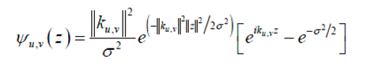
z = (x, y) and e is a function of oscillation, whose real part is the cosine function and imaginary part is a sine function.
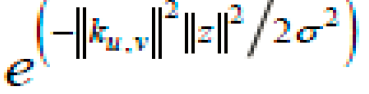 is the Gauss function. The Gauss window reflects the localization of the Gabor filter both in the time and frequency domain, and limit the range of the oscillation function. Gabor filter can tolerate slight image distortion by using the Gauss window.
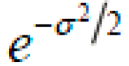 is the DC composition which can be deduced to make the wavelet DC free. kμ,v is the wave-vector of the filter corresponding to orientation μ and scale v . Through choosing a series of kμ,v a set of Gabor filter can be obtained. σ is a constant that portray the wavelength of the Gauss window. Here I choose σ = 2π. kμ ,v can be further written as
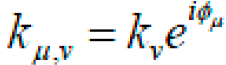
where kv = kmax / f v and φμ = πμ / 8. kmax is the maximum frequency, and f is the spacing factor between kernels in the frequency domain. Different v is chosen to describe different wavelength of the Gauss window, and then control the scale of sampling. Different μ is chosen to describe the oscillation function with different direction, and then control the orientation of sampling. In this work, I use Gabor wavelets at five different scales, v ∈{0,...,4}, and eight different orientations, μ ∈ {0,...,7}. Five scales and eight orientations generate 40 filters. Figure 1. shows the real part of the 40 Gabor kernels with the following parameters: σ = 2π, kmax = π /2 and f = 21/2. The wavelets exhibit desirable characteristics of spatial frequency, spatial locality and orientation selectivity.

Figure 1. The real part of the Gabor kernels at five scales and eight orientations
The Gabor wavelet representation of an image is the convolution of the image with a family of Gabor wavelets. I convolve the image with complex Gabor filters in 5 spatial frequency and 8 orientation so that the whole frequency spectrum, both amplitude and phase can be captured. After convolution, local features can be represented by a set of convolution results at a certain convolution point which contains the important information at different orientation and scales. In Figure 2, an input vehicle image and the amplitude of the Gabor filter responses are shown.
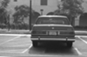
Figure 2(a). Original vehicle image
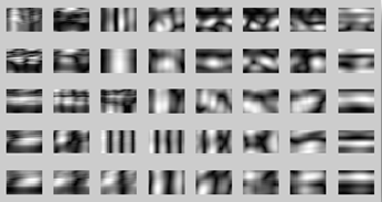
Figure 2(b). Filter response
Feature Extraction
I design artificial neuron network which prepares images for training phase. All data from both “vehicle” and “non-vehicle” folders will be gathered in a large cell array. Each column represents the features of an image while rows consist of file name, prepared feature vector for the training phase, and corresponding desired output of the network.
I adjust the histogram of the image for better contrast. Then the image will be convolved with Gabor wavelet by multiplying Gabor filters. However, despite the advantages of Gabor wavelet based algorithms in recognizing vehicle images with different illumination, scale and orientation, they require high computational efforts. The process of the convolution of a 21*32 pixel image with 40 Gabor wavelets remains a time consuming step and would become the main computation overloads for vehicle detection algorithm. Therefore, I use Fast Fourier Transform (FFT) and Inverse Fast Fourier Transform (IFFT) to speed up the computationally intensive convolution process, i.e., both Gabor wavelets and the image are transformed to frequency domain using FFT and the product is then transformed back to spatial domain using IFFT.
To save time, the family of Gabor wavelets has been saved in frequency domain before the convolution of the image. After performing convolution, the 40 Gabor filtered images are concatenated together to form a big 105*256 matrix of complex numbers which means that the dimension of the extracted Gabor feature would be incredibly huge, i.e., 26,880 for images with size 21*32 when 40 wavelets are applied. Consequently, dimensional reduction technique is used to reduce the dimension to a certain magnitude.
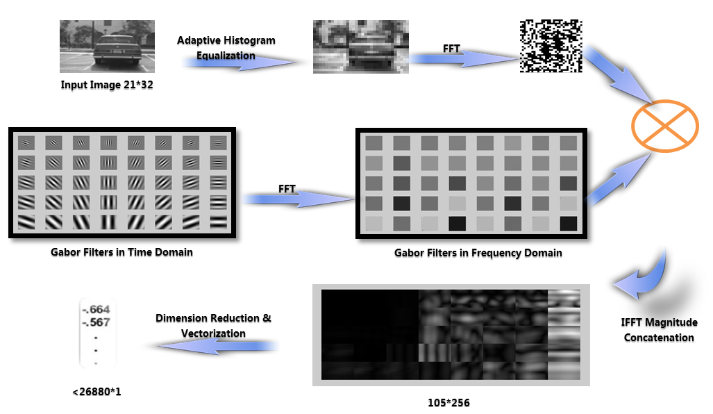
Figure 3. Steps involved in feature extraction
Classifier training
Once the dimension of an extracted feature vector has been reduced and discrimination ability enhanced by a certain subspace analysis, artificial neural network classifier could be applied for classification. The Multi-layer Perceptron (MLP) neural network has feed forward architecture with an input layer, a hidden layer, and an output layer. The input layer of this network has N units for an N dimensional input vector. The input units are fully connected to the hidden layer units, which are in turn, connected to the J output layers units, where J is the number of output classes.
In this work, I implemented a 3-layer feed forward neural network. The input layer is constituted by 3010 neurons because the dimension of the feature vector has been reduced to the same size. The network also has one hundred neurons in the hidden layer and one neuron in the output layer. The single neuron in the output layer is active to value 1 if the vehicle is presented and 0 otherwise.
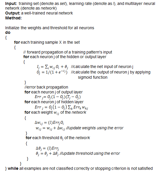
A feed forward Backpropagation learning algorithms was chosen for the proposed system because of its simplicity and its capability in supervised pattern matching. Our problem has been considered to be suitable with the supervised rule since the pairs of input-output are available. The Backpropagation algorithm implemented on training network can be summarized as follow:
- Initialize the network weights to random numbers between -0.5 and 0.5
- Initialize the thresholds for all neurons to random numbers between 0.25 and 1
- Apply normalized input to the network
- Calculate the output using sigmoid function
- Compare the resulting output with the desired output for the given input and compute the difference of desired output and actual output (which is also called error)
- Propagate the error signal from output layer to hidden layers to input layer
- Revise the weights and thresholds for all neurons using the error
- Repeat the process until error reaches an acceptable value which means that the network is trained successfully, or if we reach a maximum count of iterations, which means that the training is not successful
The above algorithm summary can be converted to pseudocode below:
Feature Point Localization
After training neural network, I perform classification method for testing image. To reduce computational complexity, feature vectors are extracted only from points with high information content on the testing vehicle image. We do not fix the locations or the number of feature points in this work. The number of feature vectors and their locations can vary in order to better represent diverse characteristics of different vehicles. The above mentioned high-energized points could be pinpointed by the following method.
A feature point is located at (x0, y0), if
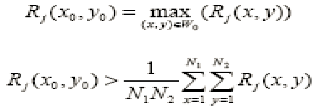
where Rj is the response of the testing image to the jth Gabor filter. N1, N2 is the size of vehicle peaks of the responses. In our experiments a 9*9 window is used to search feature points on Gabor filter responses. As the samples of Gabor wavelet transform at feature points, feature vectors represent both the spatial frequency structure and spatial relations of the local image region around the certain feature point.
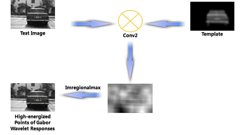
Figure 4. Steps involved in feature point localization
Image Scanning
In this step, the algorithm will check all potential feature points and the windows around them using neural network. The result will be the output of the neural network for checked regions. The procedure goes as follows:
- Filtering above pattern for values above threshold
- Dilating pattern with a disk structure
- Finding the center of each region
- Draw a rectangle for each point
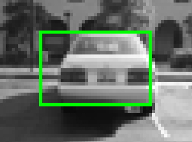
Figure 5. Vehicle detection process
Results
To evaluate the performance of the proposed approach, the average accuracy (AR), false positives (FPs), and false negatives (FNs), are recorded.
For testing, I use a fixed set of 200 vehicle and non-vehicle images which are extracted from the MIT CBCL car database. First, I compare three different Gabor filter banks, one using 5 scales and 8 orientations, one using 4 scales and 6 orientations and one using 3 scales and 5 orientations. Figure 6 and Figure 7 shows the average AR, FPs, and FNs for each case. It is interesting to note that the second filter bank yield higher FNs while the third filter bank yield higher FPs though the AR is almost the same in both cases. Obviously, the number of scales and orientations need to be chosen carefully for optimum performance.
Then, I compare the performance of neural network classifier with SVMs. SVMs outperform neural network. In particular, the SVM classifier achieves approximately 5% higher accuracy using Gabor features. Moreover, SVM based vehicle detection approach is faster while Backpropagation algorithm takes longer time to converge.
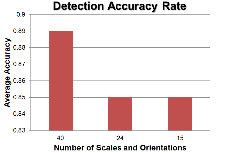
Figure 6. Average AR for different gabor filter bank
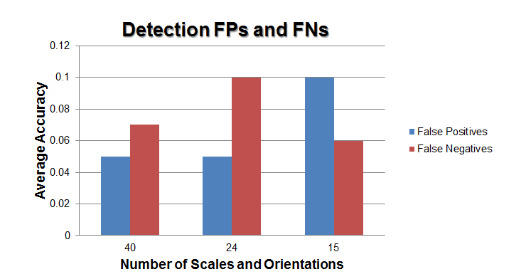
Figure 7. FPs and FNs for different gabor filter bank
Conclusions
In this work, an approach to vehicle detection with Gabor wavelets and feed forward neural network is presented. From the experiments, it is seen that proposed method achieves satisfactory recognition results. Proposed method is also robust to illumination changes as a property of Gabor wavelets, which is the main problem with many other approaches. In order to further speed up the algorithm, number of Gabor filters could be reduced with an acceptable level of decrease in detection performance.
References
- N. Matthews, P. An, D. Charnley and C. Harris, “Vehicle detection and recognition in greyscale imagery”, Control Engineering Practice, vol. 4, pp. 473–479, 1996
- Z. Sun, G. Bebis and R. Miller, “On-road vehicle detection using Gabor filters and support vector machines”, IEEE 14th Int. Conf. Digital Signal Processing, Greece, pp. 1019–1022, 2002
- Z. Sun, G. Bebis and R. Miller, “On-road vehicle detection using evolutionary Gabor filter optimization”, IEEE Transactions on Intelligent Transportation Systems, vol. 6(2), pp. 125-137, 2005
- Yang Zhang, “Time Frequency Analysis Tutorial: Gabor Feature and its Application”
- Linlin Shen, Li Bai, “A review on Gabor wavelets for face recognition”, Pattern Analysis and Applications, vol. 9(2), pp. 273-292, 2006
- MIT CBCL Car Database, http://cbcl.mit.edu/software-datasets/CarData.html