Flocking behavior of US equities
Ira Ray Jenkins and Tim Pierson
Dartmouth College Department of Computer Science
{jenkins, tjp}@cs.dartmouth.edu
Abstract
Can we predict stock prices if the market is modeled after a flock of animals? It was once thought impossible to predict the behavior of flocking animals. However, biologists have identified a small number of features, such as the speed and direction of individuals within the flock, that can model the dynamics of the flock with some accuracy. Similarly, many in the past have suggested the markets are unpredictable. We explore the possibility of predicting the behavior of the stock market based on features analogous to those developed by biologists. Specifically, we attempt to model an industry sector as a flock, with the companies within that sector as the individuals within the flock. We have modeled two approaches for this problem. First, a two-phase neural network for predicting any stock's future movement. Second, a genetic algorithm designed to identify potentially advantageous feature values where accurate predictions might be possible. The two-phase neural network had disappointing results; however, the genetic algorithm was able to identify a few key areas of potential prediction that leads to fairly accurate results.
Introduction
Modeling the behavior of flocks of animals
Accurately modeling the collective behavior of large groups of animals has historically been difficult [1,3]. Early attempts to model flock behavior with computer generated "boids", however, uncovered three basic rules for each individual in a flock that can produce realistic computer simulations of flocking animals [12]. These rules are:
- Collision Avoidance. Avoid collisions with nearby flock mates.
- Velocity Matching. Attempt to match velocity with nearby flock mates.
- Flock Centering. Attempt to stay close to nearby flock mates. (Animals outside the flock tend to get eaten.)
More recent studies of animal flocking have built upon these rules, refining the concept of Collision Avoidance into the concept of a Zone of Repulsion around each animal, Velocity Matching into a Zone of Orientation, and Flock Centering into a Zone of Attraction [4]. See Figure 1 for more details.
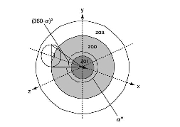
Figure 1.
A representation of an individual in three-dimensional space, centered at the origin and pointing in the direction of travel. The area labeled zor shows the Zone of Repulsion where individuals try to avoid collisions. The area labeled zoo represents the Zone of Orientation where individuals try to align their direction of travel with neighboring individuals. The area labeled zoa is the Zone of Attraction where individuals attempt to stay close to others in the flock. A possible "blind volume" behind each individual is also shown. An individual's field of perception is indicated by α. [4]An animal's position relative to other animals in each Zone provides clues as to what action an individual will take. For instance, in a flock of birds, if a neighboring bird enters into the Zone of Repulsion of Bird A, perhaps because it was caught by a gust of wind, then Bird A will maneuver away from that neighbor to avoid a collision. This in turn may effect Bird A's other neighbors, causing animals on Bird A's left to maneuver left. Continuing on, birds in the Zone of Attraction will attempt to stay close to the maneuvering birds, and may also move left. This maneuvering may cause the flock to make a change of direction that was originally based on the action of a single bird trying to avoid a collision.
These rules work well if we imagine a predator approaching a flock. Individuals on the perimeter of the flock may notice the predator and maneuver away from the threat. This causes the birds near the outside of the flock to maneuver away from the birds reacting to the predator (in this case to avoid collision). This reaction quickly ripples through the entire flock and results in the entire flock moving away from the predator almost instantaneously. Interestingly, this action is intelligent for the flock, but happens without a leader directing the individuals and with each individual having only local knowledge of the environment (e.g., individuals do not have knowledge of the location and actions of every individual in the entire flock). Our suspicion was that equities do something similar. There is no leader directing the movement of individual equities in the stock market and the market tends to react quickly to events such as breaking news.
Modeling the equities markets as a flock
In the past it was considered impossible to predict direction changes in a flock of real animals, but Bialek has recently reported good success [2]. Similarly many consider it impossible to accurately predict changes in prices of equities in the stock market [8]. We hope we will be able to use the principles others have used to predict the movement of flocks of animals to accurately predict the movement of equity prices in the stock market.
In our case, we will use individual stocks to simulate individual animals and will use industry sectors to simulate flocks (e.g., the individual company Apple belongs to the Technology sector or flock). During the course of the term we developed metrics to simulate an individual's position within the flock. For instance, we modeled the percentage change of a stock's current price vs. the closing price of the previous trading day. When we looked at all stocks within an industry sector, we saw some stocks up in price, some down in price, and some relatively unchanged. This then gave us an indication of each stock's position within the flock. The direction each individual animal was facing was simulated by the recent price changes of each equity (e.g., the price over the last n minutes has been going up, so the individual is facing upward, or the price has been going down, so the individual is facing downward). The velocity of each individual was modeled by recent volume of trading activity.
Our hypothesis was that there are times in the market where prices are changing in a predictable fashion, akin to a flock of animals moving predictably away from a predator. The cause for united movement of the flock in the equities markets may be due to a number of factors including breaking news that affects the entire market, specific sectors or just specific stocks. We hoped, for instance, that the metrics we developed would allow us to determine that a particular stock or sector is moving, then accurately predict the movements of other stocks in response. This is similar to how biologists are trying to predict the movements of individuals animals based on movements of nearby animals in the same flock.
We also expected that there would be times when the markets exhibit behavior described by the well–known Random Walk Theory [7]. In these cases, the stock market is not moving predictably in any particular direction. Instead the market is floating up and down, with prices of each equity changing by small amounts in a relatively random fashion. This behavior, we hoped to find, is similar to a flock of animals milling about, with each individual animal moving in random directions, but staying close to the center of the flock. We hoped the metrics we developed would help us identify these times when price changes are moving randomly and unpredictably.
We realized that modeling stocks within a sector is not exactly like modeling individual animals within a flock. We suspected, for instance, that there is no Zone of Repulsion for in the equities markets. Real animals cannot occupy the same space at the same time and try to avoid collisions. Stocks, however, can have the same price. To be clear, we were inspired by the work of biologists on flocking behavior of real animals and hoped to use it as a starting point to learn more about the behavior of equity markets.
Challenges
Equities markets are notoriously difficult to predict. In fact, the famous Efficient Market Hypothesis (EMH) suggests that it is impossible to predict the direction of equities markets because the market price of each individual equity already accounts for all known information. Furthermore, the EMH states that prices change instantly to reflect new information [8]. If the EMH turns out to be perfectly accurate, then our approach could yield no tangible results. There is, however, a good deal of evidence to suggest the EMH is not completely accurate [14].
Methods
Developing the feature set
Separate companies into flocks according to industry sectors
Our idea was to model industry sectors as flocks of animals and individual companies within the sector as individual animals within a flock (e.g., 3M is in the Industrials "flock"). We had data on stocks (obtained privately by one of the team members) in the Standard and Poor's 500 Index (S&P 500) and we used the industry classifications that S&P uses to categorize companies into groups. This gives us 10 flocks:
- Energy
- Materials
- Utilities
- Consumer Staples
- Industrials
- Financials
- Information Technology
- Telecommunications
- Health Care
- Consumer Discretionary
Focus on a particular flock — Industrials
We had data on the open price, high price, low price, close price, and volume in one-minute increments for the 500 stocks in the S&P500 for two years. This gave us over 2.3 billion features we could develop (500 stocks * 390 minutes/trading day * 252 trading days/year * 2 years * 24 features). To reduce this size we decided not to try to model all flocks at one time, but instead chose to initially focus on one sector.
We decided to initially focus on the Industrials sector for a number of reasons. First, our suspicion was that because the Industrials sector is less volatile than other sectors such as Technology or Energy, that it might be easier to make accurate predictions.
Another reason to choose Industrials is because we had data for the entire period for 63 individual stocks. In some sectors, such as Technology, companies join the S&P 500 Index and leave the S&P 500 Index more frequently (e.g., Facebook joins the Index, while last year's darling leaves the Index). We considered that the relatively large number of companies in the Industrials sector that stayed in the index for the entire period should help mitigate any unusual behavior of any particular company.
Model each company
Having elected to focus on Industrials, one possible course of action would be to build a model for each company within the flock. While this approach might make a lot of sense, for example General Electric's stock probably does not behave exactly like ADT Corporation's stock, we chose not to take this approach. With the choice of the Industrials sector, our hope was to minimize volatility (outliers) and produce a suitable flock-wide model that would perform well.
Developing features based on biological flocks
Biologists have identified a number of features that model the dynamics of animal behavior within flocks. See Figure 2 for examples of emergent behavior.
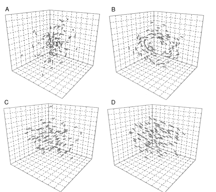
Figure 2.
Factors such as group polarity (e.g., the degree of alignment of individuals) and group velocity (e.g., how fast the group is moving) which are derived from characteristics of each individual animal can lead to the emergence of different behavior for the flock as a whole. Figure A show a "swarm" of animals milling about with low polarity and low velocity. Figure B shows a "torus", a flock with low polarity and high velocity. Figure C shows a "dynamic group", with high polarization and high velocity. Figure D shows a "highly parallel group" with high polarization and low velocity. From Couzin and Krause, 2003 [3].Inspired by the biologist's work, we developed 25 features that have some analog to natural flocks. Some of the common features that biologists use in their models are:
- Position of an individual. Biologists use 3 dimensions for birds and fish and 2 dimensions for earth bound animals like wildebeest. We model stock position as 1-dimensional — the percentage change in price from the previous night's close. In our case, some stocks will be up, some will be down. We use percent change, as opposed to absolute change in dollars because stocks have varying prices. For example, a $700 stock that moves 1% will move $7. However, that same $7 movement would be a 70% move for a $10 stock. By using the percent change we normalize this concept and make it easier for the model to deal with.
- Velocity of an individual. Biologists use the animal's actual speed. We are using the number of shares traded (see below for difficulties in this) to represent velocity.
- Rank of an individual. In some biological groups individuals have different social rank and can influence the group's behavior more than others. Think of a lion pride, where one lion is the "king" and can influence the actions of other lions more than a lion of lower status can influence other lions. We model this effect by including the market capitalization of the individual stocks.
- Direction an individual is facing. Biologists can use a compass heading based on the direction the animal's nose is pointing. We are using the slope of a linear regression of the recent stock prices. In our case, some stocks will be pointed up (e.g., prices have been increasing as indicated by a positive regression slope) or pointed down (e.g., prices have been decreasing as indicated by a negative regression slope), or pointed straight ahead (e.g., indicated by a close to zero regression slope).
- Center of the flock. Center point of all animals in the flock. We model this as the average change in price from the previous night's closing price of all individuals in the flock.
- Velocity of the flock. How fast the center of the flock is moving over time. We model this as the average velocity of individuals in the flock (see below for difficulties in modeling this).
- Direction of the flock. This is the change in coordinates of the center of the flock over time. We model this as the average direction all individuals are facing.
- Polarity of the flock. This is how aligned individuals are in the flock. In some instances individuals are milling about, facing in different directions (see Swarm in Figure 2 above). In those cases, the group's polarity is low. In some cases the group is moving purposefully in a specific direction. In this case, the group has high polarity. We are modeling polarity as the standard deviation of the direction all individuals are facing (e.g., are they all going up, or all going down, or relatively flat). A low standard deviation suggests a high polarity.
- Flock density. This is how tightly packed the flock is. We model this as the standard deviation of the position of all individuals. As described above, the position of each individual is the percentage change in price from the previous night's closing price. A low standard deviation of all individuals' positions suggests a high density.
- Time of day. In the real world, animals behave differently at different times of day. For example, some animals sleep during the day and are active at night (like grad students?). Others are reversed. We model difference in behavior at different times of the day by providing the model the number of minutes since the market opened for each feature.
Below is a brief summary of our model features, grouped by stocks and sectors, and their biological analog.
| Biological Feature | Market Feature |
|---|---|
| Individual Stocks | |
| Position | Percent change in price from previous night's close |
| Velocity | Z-Score of number of shares traded per minute for the current minute and previous four minutes |
| Rank | Market capitalization |
| Direction | Linear regression slope of recent prices for 1, 5, 10, and 20 minutes |
| Sector "Flocks" | |
| Center | Average change in price from previous close of all individuals |
| Velocity | Average of velocity of all individuals for current minute, plus previous four minutes |
| Direction | Average of direction all individuals have been facing for 1, 5, 10, and 20 minutes |
| Polarization | Standard deviation of direction of all individuals for 1, 5, 10, and 20 minutes |
| Density | Standard deviation of change in price from previous close of all individuals |
| Time | Minutes since the market opened |
Difficulty modeling some features
Some features were difficult to model. For instance, we wanted to model the velocity of particular individual as the number of shares traded recently. But, two issues confounded that. First, volume is very inconsistent. For example, in Figure 3 below we see a big change in the volume of shares traded each minute. This happens very commonly in the market.
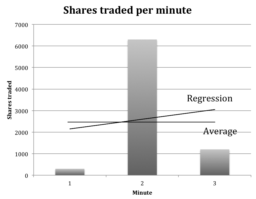
Figure 3.
Variance in shares traded. This figure shows how the number of shares traded per minute can vary substantially over a short period of time. Here we show the number of shares traded for a particular company over a three-minute period. The question then is how to model this. One approach might be to take the average number of shares traded. This approach, however, may not be a good indication of the velocity. Another approach might be to do a linear regression over a small time period and use the slope. Again, this approach might not serve a model well.Our approach is to first calculate a Z-score for each minute of trading. This is calculated by first determining the average number of shares traded per minute of each trading day (this varies considerably during the day, where right after the market open and right before the market close average share volume is typically much higher than during the middle of the day) and the standard deviation of the number of shares at each minute. Then for each sample, we take the current shares trades and subtract the average shares traded for that minute. We divide this by the standard deviation of the number of shares traded.
Where:
v = volume for this minute of the trading day
μ =
average volume for this stock for this minute of the trading day
σ = standard deviation for this stock for this minute of the
trading day.
In this way we normalize a score for all stocks, whether they trade relatively high volumes or whether they trade relatively low volumes.
Once the Z-score is calculated, we provide the model with the current Z-score and the previous four minutes' Z-scores (a total of five minutes). In this way we let the models determine what is most important, rather than providing a summarized metric such as the average score or slope of a linear regression of volume traded over five minutes.
Developing target values
We are trying to predict the movement of stock prices based on what the flock is doing at any particular point in time. One natural question that arises then is how far into the future should we predict. We decided to develop targets that are the percentage change in price (so we can more easily handle difference in the magnitude of stock prices, $700 vs. $10) for 1, 5, 10 and 20 minutes into the future. The Efficient Market Hypothesis tells us the price in the near future should be the price it is currently, but we see clearly that prices will drift more over longer periods of time. Our presumption is that it will be easier to accurately predict the price 1 minute into the future than it will be to predict 20 minutes into the future. Nevertheless, we developed targets for each of these time periods to investigate temporal effects.
Neural Network
Test results looked promising at first, then reality set in
Because our data is a time series, we first decided to investigate Matlab's time series Neural Network tools. We initially selected the Nonlinear Autoregressive with External Input (NARX) tool and ran it with our data. The results were spectacular (see Figure 4 below).
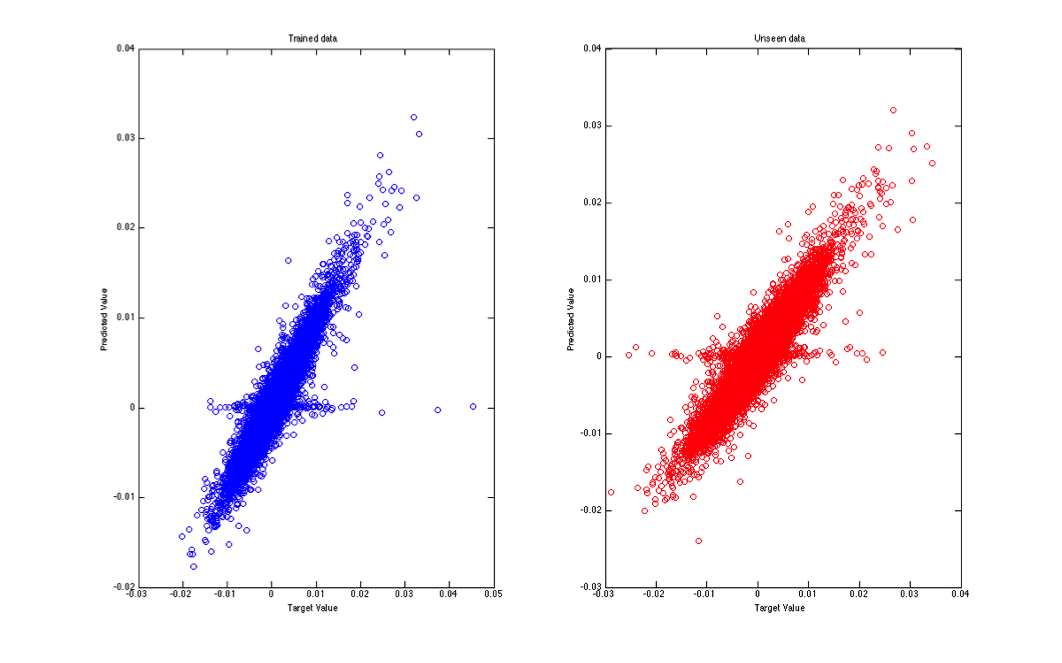
Figure 4.
NARX results. This figure shows the performance of the NARX neural network on roughly 100,000 samples while trying to predict price changes 20 minutes into the future. The x-axis shows the actual target value (e.g., the price 20 minutes in the future). The y-axis shows the model's predictions. The left figure shows performance vs. training data. The right figure shows performance vs. testing data. If the model were perfectly accurate the points would align at a 45-degree angle. This shows performance very close to that.As we dug deeper into how NARX networks work, we realized we had a problem. In the NARX topology, target values are fed back into the model, making it a recurrent model. In our case, however, y(t) is the value of the price change some time period in the future. Here the time period was 20 minutes. See Figure 5.
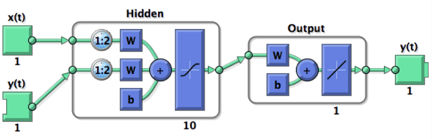
Figure 5.
NARX Neural Network. Diagram of a NARX neural network. Notice that the true values of the targets, y(t), are fed into the model. In our case this would be the price change 20 minutes into the future lagged by one minute, giving the model the chance to make a prediction of the price change 20 minutes into the future using the price change 19 minutes into the future as an input. Graphic from Matlab documentation.A closed loop version of the NARX network could use the predicted value (e.g., model output, not the true value) of the previous minute as input into the next prediction and this may be an area to examine in future work. We decided to use a non-recurrent version of the Matlab Neural Network Toolbox to make sure we've eliminated this potential complication.
When we ran the model again using the Matlab Fitting Tool to perform a regression against the change in price 20 minutes into the future, we saw a remarkable decrease in performance. Reality had set in. Our network wasn't performing as well as we'd hoped. See Figure 6.
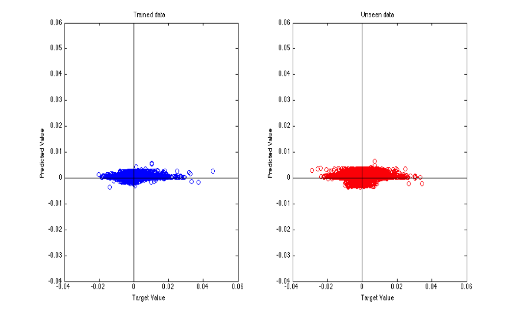
Figure 6.
Matlab Neural Network Fitting Tool performance. This figure shows the performance of the Matlab Neural Network Fitting Tool on roughly 100,000 samples while trying to predict price changes 20 minutes into the future. As before, the x-axis shows the actual target value and the y-axis shows the model's predictions. The left graph shows the performance against training data. The right graph shows the performance against test data. In both cases the predicted movements are close to zero.When we reviewed the target data more closely, we saw the culprit. The vast majority of inputs, even when looking 20 minutes into the future showed near zero movement. See Figure 8.
The fact that relatively large price changes are uncommon, even when looking 20 minutes into the future means our model was able to do a reasonably good job overall if it predicted nearly no movement. This stands to reason. If 99% of the time there is no movement, then simply predicting no movement means the model will be accurate 99% of the time. That, however, is not useful for our purposes. We are specifically looking for cases where the stock will reliably have a significant price change
New approach — model this as a two-stage problem
After speaking with Prof. Torresani, we came up with a new plan to overcome these obstacles. We modeled this as a two-stage problem. The first stage was to train a neural network to detect if the stock will have a reasonably significant price change over the next few minutes. This stage simply output one if the stock was predicted to move, it could move either up or down, otherwise it output zero. The second stage predicted which direction the stock would move, up or down, only if the first stage predicted a significant price change. In a sense the first stage provided a filter for the second stage.
First stage — predict if there will be a significant price change
The first stage's task is to predict when a stock will make a significant price change. We modeled this as a classification problem, whereas previously we'd modeled it as a regression problem. That is to say, previously we were predicting the percentage change in price as a real value, we switched to predicting a class of type one if the price will make a significant move and a class of type zero otherwise.
Three questions naturally come to mind given this approach:
- What constitutes a significant price change? We decided to use 0.5% as a threshold denoting a significant price change. This choice was not entirely arbitrary, but was also not entirely rigorously selected. We could use a smaller move, but we are concerned that it would result in more noise for the model to contend with. With a smaller value for a significant price change, if the stock were moving randomly as in the "Swarm" configuration in Figure 2 above, then sometimes the stock would randomly cross the this threshold, even though it was moving as a random walk. Using a higher threshold helps to prevent that. Using a value that is too high, however, would reduce the number of samples that actually make the move. For instance, looking one minute into the future, approximately 0.3% of samples have a price change at our level of 0.5%. Increasing the required move would result in fewer samples displaying a significant move and give the model less data to use to discriminate between movers and non-movers.
- How far into the future should we try to predict? After the milestone, we saw that shorter time periods with smaller networks yielded better results. See Figure 7 below. We built upon this in our subsequent experimentation.
- How many neurons should be in the hidden layer? Another issue is network configuration. A smaller network, with a smaller number of neurons in the hidden layer, will likely be more resistant to over fitting, but might not have enough computational power to discern subtle signals of an impending price change. To understand this, we ran models to evaluate how many neurons to use. See Figure 7 below.
To better understand issues 2 and 3 above, we used 5-fold cross validation against our training data. It should be noted that a single run took about 18 hours. Because we had 7 million rows of inputs and targets, and we wanted to try multiple time periods and network configurations (and we need to use our computers for other class work), we randomly sampled our data to test the various setting. The following is pseudo code for our effort to choose our configuration optimally:
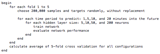
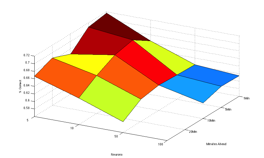
Figure 7.
Surface plot of various configuration options. This figure shows the number of neurons in the hidden layer on the x-axis and the number of minutes ahead to predict price changes on the y-axis. The percentage of correct model outputs where a class of one is predicted is show on the z-axis.One important point about this surface plot involves the values on the z-axis. In a real-world stock-trading situation, we would be most concerned about cases where the model predicted a significant price movement, but none occurred. We might use the model's output as a signal to buy shares in a company. If it failed to move, we would not make a profit (although we would not loose much money). As a result, we plot on the z-axis the percentage of time the model predicted a significant price movement and a significant price movement actually occurred. The model outputs a value in the range [0,1]. Currently if the value is greater than 0.5 we declare the output to predict a significant price movement. This value, however, could be adjusted so that the model will would have to be more confident before we declare a likely significant price movement. We could, for instance, set this threshold to 0.75. In this way the model would predict a fewer number of significant price moves, but it would be more confident when it does.
In the interest of completeness, there is another type of error the model could make that we are less concerned about. The model could predict that the stock would not experience a significant movement over the time period, and a significant movement could occur. In a real-world stock-trading situation, we could view these cases as an opportunity cost. We missed the opportunity to take part in a price movement, but we are less concerned because we would not have put capital at risk. Ideally, however, our model would catch most of these instances and alert us to the possibility of a significant price movement.
In the end, there is a trade-off to be made between making a smaller number of more accurate predictions or a larger number of less accurate predictions. Either case could be profitable. For example, making a stock trade one time per week and getting it right 100% of the time with a profit of 0.5% at each trade would be less profitable over time than making one stock trade per day and getting it right 80% of the time on average.
Second stage — predict the direction (e.g. up or down) of a significant move
The second stage's task is to predict which direction a stock will move. We also modeled this as a classification problem. If the first network predicts a significant move, again determined by our 0.5% threshold, then the sample that is predicted to move will be fed into the second network as input. The second network was trained on only examples that did move. The idea being, if it only knew about examples that moved, it would be able to detect the pattern of direction when given an example that moved.
Results
Hyper-Parameter Selection
We reviewed the results presented during the milestone that suggested a 1-minute look-ahead and a 5-neuron network. The previous results were obtained with a single run of 100,000 samples. We decided to increase our sample size to 1,000,000, to get a more accurate view of our complete data set, and we performed 10-fold cross-validation to verify our results. Those results are shown in Figure 9.
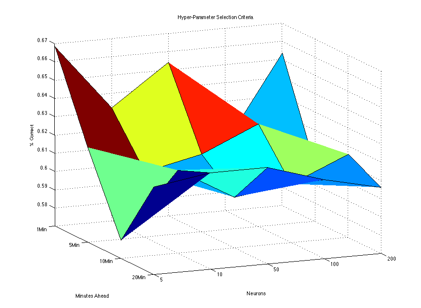
Figure 9.
Surface plot of various configuration options. This figure shows the number of neurons in the hidden layer on the x-axis and the number of minutes ahead to predict price changes on the y-axis. The percentage of correct model outputs where a class of one is predicted is show on the z-axis. The best performance was on shorter time periods.Again we saw that the neural network seemed to perform well with 1-minute look-ahead and a 5-neuron network. In the interest of time, we could not run all network configurations again on both phases. We did elect to run networks of sizes 5 and 50-neurons, both at 1-minute lookaheads.
Phase One Results
The first network, to predict stock movement, was a flop. We could show a confusion matrix of the results; however, with 10-fold cross-validation, the first network still predicted no movement nearly 99.9% of the time. We examined our data sample for the training and testing phases of this single neural network in an attempt to identify the issue preventing it from making any predictions, even in the face of samples that moved. Provided with a balanced or nearly-balanced input for training of samples that made no movement or some movement, the network continued to fail to discriminating between the two. Reducing the sample size from 4 million samples to 10 thousand samples increased the accuracy by a small amount; however, it was still effectively guessing each test example that it saw, achieving between 45% and 53% accuracy on the best runs.
Phase Two Results
In separate testing of the second network, to predict the direction of the stock movement, we trained on samples that showcased significant movement (greater than 0.5%). We found that we had trouble finding enough samples within our data set that moved beyond that threshold. Out of 4 million total samples read by Matlab, only around 100,000 samples moved more than the 0.5% threshold. We anticipated that this would be enough; however, again, we discovered that the neural network was no better than just simply guessing, with accuracy between 47% and 52% on the best runs.
Transitioning to a New Approach
There could be many issues with our neural network approach. For one, we set our movement threshold to 0.5%. As is shown below, the genetic algorithm actually shows that a smaller threshold of around 0.2% would have been better on our data set. Another issue may be our selection of sector. Related to the movement threshold, we chose the Industrials sector because we thought it would showcase little volatility (unlike other sectors like Technology). This might have been a flawed approach in light of our movement threshold of 0.5% because the sector and the companies within it simply do not vary widely. Also, in comparing our approach with those typically used, we only modeled the sector as a flock and chose not to model individual companies within that sector. It might be possible to model both and achieve better results. In an effort to find a method that would produce more favourable results, and in light of Prof. Torresani suggesting we implement our own algorithm, we transitioned to a genetic algorithm.
Genetic Algorithm
Looking for areas of predictability with a genetic algorithm
With the neural network approach we were looking for a solution where we could make an accurate prediction regardless of the input vector. What we quickly realized, however, is that most of the time the stock price does not change very much. See Figure 8 below.
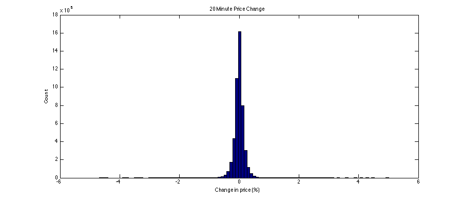
Figure 8.
This diagram shows a histogram of the change in price over a twenty-minute period. The x-axis is the percentage change in price and the y-axis shows a count of the number of instances with that change. Clearly most of the time the price does not significantly change.Because most of the instances had little change in price, we reasoned that our neural network would spend a great deal of its computational power focused on areas with little price change because the overwhelming majority of our training data had little price change. For our purposes, however, we are most interested in focusing on situations where the price will change significantly. We wondered if we could find areas of predictability in the input space where we could reliably predict large price movements. In other words, we wondered if instead of trying to create a model that would perform well regardless of the input feature, we decided to try to find subareas within the input space where we could make accurate predictions of large price movements when a specific set of criteria were met and not make predictions otherwise. We settled on a genetic algorithm to search for areas of predictability.
Basic Genetic Algorithm
The biologically inspired genetic algorithm was first introduced by Holland in 1975 [5]. In the years since there have been an enormous number of variations on the theme, but most genetic algorithms follow this basic procedure [11]:
- Start with a randomly generated population of candidate solutions (called individuals) to a problem
- Calculate the fitness, f(x), of each individual in the population
- Create the next generation:
- Select a pair of individuals for reproduction from the current population based on their fitness (e.g., more fit = more likely to reproduce)
- Create two offspring based on the selected parents
- Mutate the offspring with probability pm
- Place the offspring into the next generation population
- Repeat until the next generation population holds as many individuals as the current population
- Replace the current population with the new population
- Go to step 2
By following this procedure the algorithm attempts to evolve increasingly fit solutions to the problem. The basic idea is that by combining two fit individuals, an even more fit offspring may emerge. After a number of generations have passed the algorithm may evolve a good solution to the problem.
Previous work with genetic algorithms to find areas of predictability
We based our approach on Meyer and Packard's work using the basic genetic algorithm to find areas of predictability in blood flow using the highly chaotic Mackey-Glass equation [10]. Meyer and Packard considered input from a continuous variable sampled at discrete intervals that gave an input vector in the form:
where each xi ∈ ℜ is a sample taken at time N and the values of the previous 50 samples. Y is the target value, which in their case was the value of the Mackey-Glass equation 50 steps into the future. Their goal was to accurately predict the value of y, but only when condition when the conditions where favorable to making accurate predictions.
Meyer and Packard developed a set of conditions that allowed their algorithm to look in greater detail at discrete portions of the input space. Because each feature in the input vector was real-valued, the conditions where a set of conjunctions in the form:
A typical condition might be the conjunction:
In Meyer and Packard's genetic algorithm each individual solution contained a chromosome represented by a conjunction in the form shown above.
The fitness of each individual was evaluated by examining the standard deviation of y for those input vectors that met the conjunction, compared with the standard deviation of the entire input. They used this fitness function to evaluate all individuals:
Where:
σ is the standard deviation of y where the
conjunction was met
σ0 is the standard deviation
of y of the entire input
α is a scaling factor
N is the
number of input rows that match the conjunction.
Meyer and Packard's results suggest it is possible to predict the Mackey-Glass equation in some regions of the input space, while avoiding making predictions where it is difficult to make accurate predictions. We wondered we could adapt this approach to the stock market using our flock-inspired features as inputs.
Our implementation of the Genetic Algorithm
Like Meyer and Packard, our goal was to create a genetic algorithm that would search the input space looking for specific conditions that would allow the algorithm to make accurate predictions. In our case we were looking for large changes in stock prices t minutes into the future. In this way the genetic algorithm was not trying to make an accurate prediction for all possible input values, but instead only sought to make a prediction when the training data suggested conditions were right for the algorithm to make accurate predictions of large price changes.
Input values
Our input features were based on the idea of modeling an industry sector (e.g., Industrials, Technology, etc.) as a flock of animals and each company's stock (e.g., General Electric, IBM, etc.) as an individual within the flock. We developed 25 features to model biological flock attributes such as position, speed, heading, etc. See "Developing the feature set" above for more details.
Each input vector x was 25-dimensional with xj ∈ ℜ ∀j=1...25. We normalized these values to fall into the range [0,1] with the following formula:
Where:
xi,j = feature j of input vector i
xmin(j) = min(xi,j) ∀ i =1...m
xmax(j) = max(xi,j) ∀
i =1...m
m = number of input sample rows
n = number of
features in each row (25 in our case).
Target values
Our target values were the percentage change in stock price t minutes into the future, where t = {1, 5, 10, 20} minutes. We created separate genetic algorithms for each time frame (e.g., a single genetic algorithm did not try to predict prices at multiple time frames). At each time frame we calculated three changes in price based on: 1) the closing price t minutes into the future, 2) the lowest percent price change within t minutes, and 3) the highest percent price change within t minutes.
Our implementation of the basic algorithm
In accordance with the basic genetic algorithm described above, our algorithm worked as follows:
- Start with a randomly generated population of candidate
solutions to a problem
We created an initial population of 100 randomly generated candidate solutions according to the following pseudo code:

In this way we create an individual that has a range for each feature in the input vector like Meyer and Packard's conjunctions. We call this conjunction a chromosome. The individual matches an input vector xi if:
Individual(j)low ≤ xi ≤ Individual(j)high ∀j=1...25Where:
xij = feature j of an input vector i
Individual(j)low = low value for feature j for an individual
Individual(j)high = high value for feature j for an individual.One other thing to note with the initial creation of an individual is the wildcard operator. The wild card is a condition where feature j matches all input vectors. Because we normalized our inputs to fall in a range [0,1], we use the values of 0 and 1 for the low and high values of the chromosome respectively. The wild card option is chosen with likelihood pwc. We set pwc to 0.6.
In this way each individual serves to filter the input space into discrete subsections.
- Calculate the fitness of each individual in the
population
Getting the fitness function correct is critical to the success of a genetic algorithm. After all, each individual's chances of passing its chromosomes to the next generation through reproduction hinges on its fitness. In our case we would like the algorithm to make predictions that have the following three characteristics:
- It should predict large changes in price
- When making a prediction, the actual price moves should have low standard deviation
- A greater number of predictions is better than a smaller number of predictions (e.g., make sure the algorithm doesn't find one or a small number of conditions that have a large price change, but were just noise).
We initially experimented with a fitness function in the form:
f(x) = abs(μ/σ)*(m/m0)Where:
μ = average y of all input vectors matching the conjunction
σ = standard deviation of y of all input vectors matching the conjunction
m = count of the input vectors matching the conjunction
m0 = total number of input vectors.But function gave poor results because conjunctions that met a large percent of the input vectors dominated. For example an individual in the population that matched 1,000 input vectors was twice as fit as an individual that matched 500 input vectors. An individual that matched 2,000 input vectors was four times as fit. Unfortunately, individuals that matched a large number of inputs were also the individuals that tended to have a small price movement. In order to over come that, an individual that matched 500 input vectors would have to have an average price move four times greater than an individual that matched 2,000 input vectors. That is a tall order when we are only look a few minutes into the future.
To remedy this imbalance we reviewed the literature on multi-objective genetic algorithms (MOGAs). We knew we wanted to simultaneously optimize the three objectives listed above (e.g., predict large moves, have small standard deviation of actual price changes when making a prediction, and make many predictions). We found solutions to simultaneously optimizing multiple objectives tend to come in two flavors [6]:
- Combine each fitness function into one weighted function
- Search the Pareto-optimal front simultaneously.
Because we are not interested in large portions of the Pareto-optimal front (e.g., we are not interested in solutions that have a small standard deviation, but predict a small average price change), we settled on combining weights into one function.
With that in mind we next tried a fitness function of the form:
f(x) = 0.5* abs(μ - 0.3*(σ/σ0) - 0.2*(1-m/α)Where:
μ = average y of all input vectors matching the conjunction
σ = standard deviation of y of all input vectors matching the conjunction
σ0 = standard deviation of y of all input vectors
m = count of the input vectors matching the conjunction
α = a scaling factor (set to 500).The basic idea behind this approach was to separately weight each of the three criteria we were trying to maximize. The first factor accounted for the objective of predicting a large price change by examining the average price change of input vectors matching the conjunction. We thought this objective was the most important objective and gave it a weight of 0.5. The second term attempted to find small standard deviations of y values relative to the total input space that met the conjunction. We thought this was the second most important objective and gave it a weight of 0.3. The third term attempted to penalize the fitness if a small number of input vectors did not meet the conjunction. We used α = 500. In this way if the individual had less than 500 matches it would receive a penalty. If the individual had more than 500 matches there would be no penalty. We gave this objective a weight of 0.2.
Upon thinking about the fitness function further, we realized in a real world stock trading situation, we could tolerate a higher standard deviation if the average predicted price change was higher. For instance, if one individual solution predicted a price change of 0.25% with a standard deviation of 0.1, assuming the actual price changes are Gaussian (which they appeared to be), then about 84% of of the time the actual price change would be expected to greater than 0.15% (0.25% mean - 0.1 standard deviation). This is because in a Gaussian distribution about 68% of the samples fall within one standard deviation from the mean. That leaves about 32% of the samples in the tails. But, we would like the price move to be greater than the mean we predict, so we only have to worry about one tail. That means that 32%/2 = 16% of the time the price change would fall below the mean less one standard deviation. Otherwise, the other 84% of the time we would expect the actual change in price to be greater than the predicted mean less one standard deviation. We would lose money if the actual price changes went below 0, but the majority of the time we would make money if the mean less one standard deviation was greater than zero.
Keeping the first example individual in mind, if another individual predicted an average price change of 0.5% with a standard deviation of 0.2, we would prefer the second individual over the first, even though it's standard deviation is twice as large as the first individual. This is because about 84% of the time we would expect the price change to be greater than 0.3% (0.5% mean - 0.2 standard deviation). That would be an even greater expected profit than the first individual. That suggests we could come up with a better fitness function than the weighted approached above.
This led us to change our fitness again to account for this. We settled on:
f(x) = (abs(μ) - σ)/ymax - min(1-m/α,1)Where:
μ = average y of all input vectors matching the conjunction
σ = standard deviation of y of all input vectors matching the conjunction
ymax = the maximum observed price change in the training data
m = count of the input vectors matching the conjunction
α = scaling factor (set to 500).Now, with this fitness function we were able to look for solutions where the standard deviation can increase as the mean predicted price change increases. As a safety precaution we also divide by the maximum move possible (which is the largest price change in our training data) to make sure this first term falls between [0,1]. Finally we apply a penalty if the individual does not match at least 500 input vectors. We cap the penalty at 1.
- Create the next generation:
- Select a pair of individuals for reproduction from the current
population.
The probability of selecting an individual for reproduction is based on its fitness score (e.g., more fit individuals are more likely to be selected). Selection is done "with replacement" meaning that the same individual can be selected more than once to become a parent.
To implement this we used tournament selection with a tournament size of four. Under that scheme, four individuals are selected randomly from the population and sorted on their fitness. The individual in the tournament with the highest fitness is selected for reproduction with probability pbest (we used 0.90). If the individual with the highest fitness is not selected then another individual is randomly selected from those chosen for the tournament. In this way the individuals with the highest fitness are likely to be selected for reproduction and all individuals are likely to be considered for reproduction four times.
- Create two offspring based on the selected parents.
We used uniform crossover in our algorithm. Under this scheme a point is randomly selected between 1 and the number of genes in the chromosome (25 in our case). Two offspring are created using the following formula:
point = random(1,25)
child1 = parent1.genes(1...point) + parent2.genes(point...n)
child2 = parent2.genes(1...point) + parent1.genes(point...n) - Mutate the offspring with probability Pm.
Infrequently individuals are mutated in order to maintain genetic
diversity in the population. As in nature, most of the time mutations
are not helpful and individuals with the mutation are generally not
selected for future reproduction. Sometimes, however, a mutation
provides a benefit and creates a superior individual. In keeping with
the literature on genetic algorithms, we used pm = 0.01 as
the probability an offspring would be receive a mutation.
We created four chromosome mutation operations:
- Increase the range: this shifts the lower value down and the upper value up
- Decrease the range: this shift the lower value up and the upper value down
- Shift up: this moves both lower and upper values higher
- Shift down: this moves both lower and upper values down
- Change: if the value is a wildcard it creates a random lower and upper value, if the value is not a wild card, it makes this feature a wild card.
- Select a pair of individuals for reproduction from the current
population.
Maintaining genetic diversity
One issue with genetic algorithms is that they can lose genetic diversity. In this case the best set of chromosomes starts to take over the entire population. The result when two parents have exactly the same chromosomes is that the offspring will also have the same chromosomes. Because more fit parents are chosen more frequently for reproduction, the best chromosomes tend to be over-represented in the following generations. In that case a genetic algorithm then becomes stuck at a local minimum. Mutation can help here, but the algorithm can get stuck at a local minimum for long periods of time when solely relying on mutation.
We looked at the literature on maintaining genetic diversity and saw several approaches commonly in use including [13]:
- Adaptive mutation rate — increase the mutation as the number of generations increases to create possibly helpful genetic diversity
- Social Disasters Techniques
- Packing — of all individuals having the same fitness, only one remains unchanged; all others are fully randomized
- Judgment Day — Only a single individual with the best fitness value remains unchanged; all others in the entire population are fully randomized
- One Random Offspring Generation (1-ROG) — when two parents have the same fitness, one parent passes on to the next generation unchanged, a second, fully randomized individual is created as the second child
- Two Random Offspring Generation (2-ROG) — when two parents have the same fitness, two fully randomized individuals are created and passed on to the next generation.
We decided to use the 1-ROG approach to ensure that at least half our population had genetic material that was different from the most fit individual in the population.
Elitism
Elitism is a concept in genetic algorithms were some portion of the most fit members of the prior generation are automatically passed on to the next generation. This makes sure that superior individuals are not lost during reproduction. We used an elitism of 1. That means we passed the most fit individual from the prior generation to the next generation automatically.
Testing methods
We performed 10-fold cross-validation by creating a population of 100 randomly generated individuals, ran them according to the specifications above for 100 generations, and did that 10 times. At each fold we read in approximately 250,000 sample vectors from the nearly 7 million rows we developed previously and trained on those. After 100 generations we read in another 250,000 sample vectors and evaluated the results of the best individual on those test vectors. We did this procedure separately for predictions of the highest price and the lowest price with a time frame t = {5, 10} minutes into the future. In summary, we ran:
100 individuals * 100 generations * 10 folds * 2 price predictions (low and high price) * 2 time frames.
Results
We plotted the average predicted price of the training set and the test set for the 10 folds in our 10-fold cross-validation in figures 10 and 11.

Figure 10.
10-fold cross-validation predicting 5 minutes ahead. This figure shows the results of a 10-fold cross-validation predicting price change 5 minutes into the future. Blue lines are predictions made for the highest price the stock will reach in the next 5 minutes. Red lines are predictions for the lowest price in the next 5 minutes. The dotted horizontal lines are the results of the best individual found by genetic algorithm after 100 generations using the training data. The solid lines are the results when the same individual is run against test data it has not seen before. The horizontal line indicates the width of the standard deviation of the predicted y values and the "x" symbol represents the mean of the predicted values. The vertical dashed lines are the means of test results over all 10 folds.
Figure 11.
10-fold cross-validation predicting 10 minutes ahead. This figure shows the results of a 10-fold cross-validation predicting price change 10 minutes into the future. Blue lines are predictions made for the highest price the stock will reach in the next 10 minutes. Red lines are predictions for the lowest price in the next 10 minutes. The dotted horizontal lines are the results of the best individual found by genetic algorithm after 100 generations using the training data. The solid lines are the results when the same individual is run against test data it has not seen before. The horizontal line indicates the width of the standard deviation of the predicted y values and the "x" symbol represents the mean of the predicted values. The vertical dashed lines are the means of test results over all 10 folds.Validity
When we examine the results of our 10-fold cross-validation runs we see the training data and test data produce nearly identical results. To understand if there is a statistical difference in the mean price movements between the training data and the test data when the genetic algorithm makes a prediction, we performed two-tailed t-tests on the results. The results are summarized below:
| Time Frame | Low Price p-value | High Price p-value |
|---|---|---|
| 5 Minutes | 0.9886 | 0.9033 |
| 10 Minutes | 0.8360 | 0.9289 |
We can see clearly based on the p-values that we cannot reject the null hypothesis that the two sets are the same.
We next wondered if there was a difference in the standard deviation of the results between the training and test data. The results are summarized below when the algorithm makes predictions of the low and high price in the next 5 or 10 minutes.
| Time Frame | Low Price Std Dev | High Price Std Dev |
|---|---|---|
| 5 Minutes | 0.4863 | 0.6553 |
| 10 Minutes | 0.5326 | 0.1713 |
Again we can see clearly based on the p-values that we cannot reject the null hypothesis that the two sets are the same.
These tests suggest that our algorithm learned something about the training data (details on what it learned are below in the Conclusions section). This further suggests that perhaps we can set up a hedge fund, trade with this algorithm, and start minting money. But, maybe not. All of our data was taken from a two-year period from January 2010 to December 2012. Even though the training and test data were taken from different rows, they were still in the same two-year period. It might be the case that larger market conditions made making predictions easier or more difficult than if the algorithm were making predictions today. That is to say that we might not have uncovered the golden rules that will stand the test of time unaltered. Our strong suspicion is that certain rules work well for certain market conditions (e.g., bull or bear markets) and not well at others.
Conclusions
Even though our rules may, or may not (probably not), be universal predictors of price movements, irrespective of the larger market conditions, we can share some interesting observations we found in our runs. Before we began this exercise we expected that some of our features would be more important for making decisions than others. That turned out to be true. Here are some of the interesting observations we made based on how features were included by the individuals in the genetic algorithm.
Time of day—morning is better for accurate predictions
Making predictions earlier in the day appears to be more accurate than later in the day. Nearly all of the individuals evolved by the genetic algorithm filtered the input vector on the time of day, and nearly all of them preferred the morning. The US markets opens at 9:30am and close at 4:00pm. Most individuals would make predictions before noon.
Market capitalization doesn't matter
We expected that certain stocks would acts as leaders and other stocks, particularly smaller ones, would follow the leaders' movements. For example, if General Electric moved significantly, perhaps we could expect ADT to follow it. We did not see any evidence of this. Most of our evolved individuals did not filter at all on market capitalization.
The current volume and volume three minutes ago are important
Many of the genetic individuals predicted a movement when the trading volume three minutes in the past was low, but current volume was high. This indicates that volume has recently increased when previously it was low. Something was up with that stock!
NOTE: we normalized these scores by this formula:
Where:
v = volume for this minute of the trading day
μ =
average volume for this stock for this minute of the trading day
σ = standard deviation for this stock for this minute of the
trading day
Paying attention to the movement of the flock pays
Another commonly selected feature in our input vector was the trend of the flock over the past 20 minutes. This feature indicates if the flock is moving up in price or moving down. To calculate the flock trend, we calculated the slope of a linear regression for each stock in the flock over the prior 20 minutes, and then we took the average of all the slopes. A stock was particularly likely to have a large price move if the flock was moving up or down while the individual stock was trending in the opposite direction.
Future work
There are a large number of ways this work could be expanded. We list some of the ways below:
Evolve an individual, remove matches, evolve another individual...
We ran a 10-fold cross-validation to try to determine if there were areas of predictability in the input space. Our results indicate there might be. One approach to extending this work would be to evolve an individual solution over many generations and then remove the matching input rows from training data. Then we could evolve another individual from scratch on the remaining training data. We could repeat this process, evolving a small population of individuals, each the best individual from their generation when they were initially evolved, and cover a larger portion of the input space than one individual alone could cover. In our testing we did not do this. We simply evolved one individual over 100 generations on the entire training data.
Hill climb after the best individual is found
After a number of generations have been completed and the best individual in the population has been selected, there is a good chance that individual is not completely optimal. We could run a hill climbing procedure on the best individual to see if we could improve it. This would involve increasing the high value of each feature by a small amount, one feature at a time, and measuring the change in fitness. If the fitness is improves, keep increasing the high value until fitness stops improves. Next, for those features that did not improve by increasing the high value, decrease the high value by a small amount, one feature at a time, and measure the change in fitness. If the fitness is improves, keep decreasing. Perform the same steps on the lower value for each feature. This would allow the algorithm to "fine tune" the best individual for potentially even better performance.
Run more individuals in a population for more generations
We used 100 individuals in each population in our study. Perhaps more individuals would have achieved better results. We also ran for only 100 generations; yet often saw the algorithm evolving greater fitness in the generations near the end of the run. Given more generations, perhaps these runs would have evolved even better solutions.
Experiment with alpha
We applied a penalty in the fitness function for individuals that did not match many input rows. We used an alpha of 500. That meant that if an individual had fewer than 500 matches of training data rows, it would receive a penalty. If it had more than 500 matches there would be no penalty. Choosing 500 matches as somewhat arbitrary. It seemed like a reasonably large so that we would be less concerned that the algorithm over fit the data and learned noise. A more rigorous analysis of the value of alpha might yield individuals that score higher and are predicted more frequently.
Other industry sectors
Our experiments were conducted on data from stocks in the Industrials sector alone. Perhaps other sectors would be more or less conducive to this kind of prediction. It would be interesting to compare and contrast how a volatile sector such as technology would fair.
Other time frames
As noted above, our training data and set data were taken from the same two-year period. Perhaps this approach would not work well for time periods outside that window. It would be interesting to "shadow" trade (e.g., pretend to place actual market trades) with this algorithm on live stock market prices and observe how well it performs. If it works, perhaps we'll all retire early...
References
- Ballerini, M., Cabibbo, N., Candelier, R., Cavagna, A., Cisbani, E., Giardina, I., Lecomte, V., Orlandi, A., Parisi, G., Procaccini, A., Viale, M., and Zdravkovic, V. Interaction ruling animal collective behavior depends on topological rather than metric distance: Evidence from a field study. Proceedings of the National Academy of Sciences, 105(4):1232–1237, 2008.
- Bialek, W., Cavagna, A., Giardina, I., Mora, T., Silvestri, E., Viale, M., and Walczak, A.M. Statistical mechanics for natural flocks of birds. Proceedings of the National Academy of Sciences, 109(13):4786–4791, 2012.
- Camazine, S., Deneubourg, J.L., Franks, N.R., Sneyd, J., Theraula, G., and Bonabeau, E. Self–organization in biological systems. Princeton University Press, 2003.
- Couzin, I.D., and Krause, J. Self-organization and collective behavior in vertebrates. Volume 32 of Advances in the Study of Behavior, pages 1–75. Academic Press, 2003.
- Holland, J.H. Adaptation in Natural and Artificial Systems: An Introductory Analysis with Applications to Biology, Control, and Artificial Intelligence. Ann Arbor, MI: University of Michigan Press, 1975.
- Konak, A., Coit, D.W., and Smith, A.E. Multi-objective optimization using genetic algorithms: A tutorial. Reliability Engineering & System Safety 91(9), 992–1007. 2006.
- Malkiel, B.G. A Random Walk Down WallStreet: The Time-Tested Strategy For Successful Investing. Norton, New York, NY, USA, 2003.
- Malkiel, B.G., and Fama, E.F. Efficient capital markets: A review of theory and empirical work. The Journal of Finance, 25(2):383–417, 1970.
- Matlab. Neural Network Toolbox. MathWorks. February, 2013. http://www.mathworks.com/products/neural-network/
- Meyer, T.P., Packard, N.H., Local Forecasting of High-Dimensional Chaotic Dynamics. Nonlinear modeling and forecasting. Editors, Casdagli, M., Eubank, S., pp. 249–263. 1990.
- Mitchell, M. An Introduction to Genetic Algorithms. Cambridge, MA: The MIT.
- Reynolds, C.W. Flocks, herds and schools: A distributed behavioral model. In Proceedings of the 14th annual conference on Computer graphics and interactive techniques, SIGGRAPH '87, pages 25–34, New York, NY, USA, 1987. ACM.
- Rocha, M. and Neves, J. 1999. Preventing premature convergence to local optima in genetic algorithms via random offspring generation. In Proceedings of the 12th international conference on Industrial and engineering applications of artificial intelligence and expert systems: multiple approaches to intelligent systems (IEA/AIE '99), Ibrahim Imam, Yves Kodratoff, Ayman El-Dessouki, and Moonis Ali (Eds.). Springer-Verlag New York, Inc., Secaucus, NJ, USA, 127-136.
- Schwager, J.D., and Greenblatt, J. Market Sense and Nonsense: How the Markets Really Work (and How They Don't). Wiley, 2012.