Movie Recommender System By Tian Li, Yusheng Miao, Yaozhong Kang

What movie should you watch tonight? It's really a hard choice since there're so many movies that even scanning their brief introductions will cost us a lot of time. So we do need a personalized recommendation engine to help narrow the universe of potential films to fit our unique tastes. Fortunately, with the help of machine learning technique, it helps users to survive from enormous volume of information and provides valuable advices about what they might be looking for based on their particular information, such as profile, searching history, etc. Product recommendation on Amazon.com is one of those successful examples in this field.

As a matter of fact, there are new movies released even every day, however, comparatively few tools can hlep us organize these content and directly pick those movies that are more likely to interest us. To address this problem, we want to develop a hybrid Movie Recommender System based on Neural Networks, which takes into consideration the kinds of a movie, the synopsis, the participants (actors, directors, scriptwriters) and the opinoin of other users as well[1], in order to privde more precise recommendations.

Our recommendation process can be shown as the following diagram.

Figure 1

In addition to dataset we obtain on MovieLens, we also crawled the information of directors, writers, actors and plot key words from IMDB for each movie.

In total, we have:

100,000 anonymous ratings (in form of 1-5) from 943 users on 1,682 movies;
Each user has rated at least 20 movies;
Simple demographic info for the users, including age, gender, occupation, and zip code;
1,068 directors over all these 1,682 movies;
1,995 writers over all these 1,682 movies;
2,743 actors over all these 1,682 movies;
3,403 plot keywords over all these 1,682 movies;

In this rating-based part, we use Pearson Correlation Coefficient to find the correlation between the specific user and the rest of the users[1].

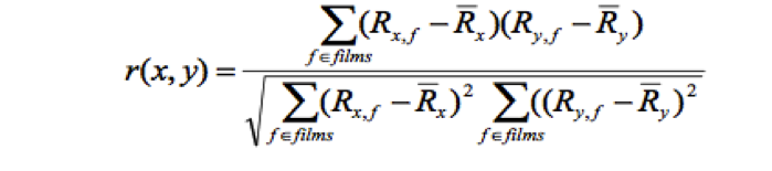
Here R_x,f is the rating of user x for film f, and

stands for the mean value of the rating of user x. Thus, for each user, we find the correlation with all the other users by applying this formula on all the movies watched by both of those two users.

The correlation we got is a decimal number that lies within [-1,1], where -1 stands for the loosest correlation between two users, while 1 stands for the strongest correlation between two users. This accords to the farthest and nearest neighbors of kNN method. In our project, we take into consideration not only the opinion of a user y who has a very strong correlation with user x, but also the opinion from a user y where he or she has a very loose correlation with user x. Because the fact shows that there is a quiet big chance that user x would like the film which disliked by user y with whom they have the opposite opinions.

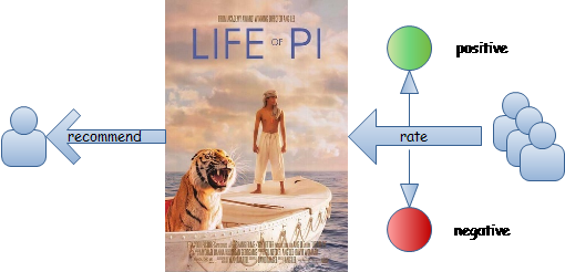
Figure 2 How counters work on a movie in the algorithm

More specifically, in our project, for each user, we assign a positive counter and a negative counter for each of all the movies. When we have a strong correlation r between user x and user y, and if user y gives a high rating on film f, then the positive counter for this specific user x on this specific movie f will be increased, which indicates that the film f has more chance to be recommend to user x. Obviously, if this user y gives a low rating on film f, then the negative counter for this specific user x on this specific movie f will be increased. As we mentioned above, in our system, we also consider the opinion from a user y who has a loose correlation with user x. Therefore, when we have a loose correlation r between user x and user y, and user y gives a high rating on film f, then the negative counter will be increased indicating that user x might like this movie which disliked by user y. Similarly, the positive counter would be increased on the opposite situation. But, in the loose correlation case, we should note that it does not necessarily mean that user x would like the film disliked by user y, therefore we give a smaller weight on both the positive and negative counters under the loose correlation situation [1].

Finally, we have two counters for each user x on each film f and we recommend films to this user x based on the values of these two counters.

In this part, we utilize the personal information of the users in our dataset. We notice that for each user, there are four attributes, age, gender, occupation and zip code to describe their personal features. We decide to use three of them to further modify our model.

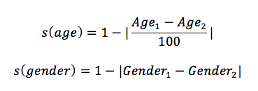
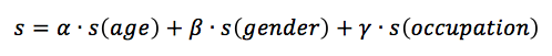
For age and gender, we can define the similarity of two persons on these two attributes as follows[2]:

In our dataset, there're 21 kinds of occupations in total. We map them to the model of 6 personality types developed by John L. Holland in Personality-Job Fit Theory[3]. (The result is shown in Table 1 [4].)

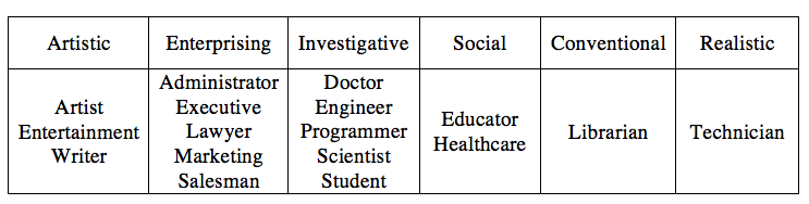
Table 1 The classification of different occupation according to Personality-Job Fit Theory.

Personality-Job Fit Theory also tells us in Figure 3, the similarity of two groups at adjacent positions are larger than those two are separated by one group, and the similarity of the latter one is larger than the two at opposite positions. Thus we calculate the distance between any two groups like this: if two occupations are exact the same, the distance is 0; if the occupations are not same but fall into the same group, we define the distance between them as 1; if the two groups are adjacent, we define distance between them as 2; if they are separated by one other group, we define their distance as 3; if they are at the opposite positions, the distance is defined as 4.

There're also four kinds of occupations (homemaker, retired, other and none) that cannot be mapped to any of these six groups, we just ignore them.

Figure 3 (Source: https://edtechvision.wikispaces.com/file/view/Holland03Jobs.gif)

Our demographical similarity can be written as follows:

When trying to recommend movies to a certain user, we use the idea of kNN to select those movies with highest average ratings by the k nearest neighbors to the user. This is based on the assumption that people with more similar background tend to share more similar interests.

The hypothesis of content-based filtering in our movies recommender system is that users would tend to like movies that are similar to those they have watched before and have given higher rates on. The similarity might be affected by many features of the movies. For example, most of us have individual preferences on certain movie types. Some of us like action movies while the others may prefer comedy. The same case appears on movie stars. Users would tend to give a higher rate to those movies acted by their favorite stars.

In additional to movie type that is included in the original dataset, we retrieved some more features about the movies from IMDB by a Web-crawler program, which is written in Java and Python. These features include:

(1) 469 actors
(2) 145 directors
(3) 688 key words

Each of these features appears in at least two movies and is represented by a vector containing 0s and 1s where 1 indicates that a certain Actor/Director/Key word is related to this movie and 0 otherwise.

We constructed three different neural networks for each user corresponding to type, actor and key words [1]. In the final result, we discarded directors because there are 61 percent of movies whose directors cannot be retrieved from the IMDB website. The same figure for actors and key words are 29% and 2% respectively.

Though we have tried to implement a neural network by ourselves, the performance is not as good as using the toolbox. After carefully inspection of this case, we found that a lot of movies are given the same prediction score. In this case, we have to choose either to recommend all of them or reject all of them where both choices do not produce good prediction result. The reason might be that the feature matrices are too sparse (an evidence is that the network constructed by type data suffers less from this problem). So finally, we present the result of this part by using the Matlab Toolbox.

The training process is based on the sub-matrix, which contains only the movies that the user has evaluated. The size of the training set varies from users since each user has rated different number of movies. Here we adopted the Resilient Back Propagation method as the transfer function in our neural network [5].

When we need to decide whether or not a movie should be recommended to a specific user, we input the three features of the movie into the corresponding network of the user. The final prediction is a weighted score based on the three outputs.

These three outputs act as a prediction of how much this user may rate the movie according to the value of the feature.

In our experiment, we use the statistical measures of a binary classification test to evaluate the performance of our algorithms. Specifically, true positive refers to the proportion of movies that our algorithm recommends and the users like as well. True negative refers to the proportion of movies that our algorithm doesn't recommend and the users don't like either. False positive refers to the proportion of movies that our algorithm recommend but the users don't like while the false negative refers to the proportion of movies that our algorithm doesn't recommend but users like. In addition, we also use precision, which is defined as the true positive divided by the sum of true positive and false negative. In the following part, we'll give out the evaluation of rating-based filtering, demographical filtering and content-based filtering respectively, followed by the performance of the hybrid method.

Rating-based Filtering

For the collaborative part, we tested the performance on different threshold and compared them in order to choose a better threshold, which can balance the number of movies we recommend and the precision rate.

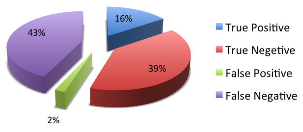
Figure 4: The percentage of four different criteria under collaborative filtering.

The figure above shows the percentage of four different criteria when threshold equals to 10. As we can see, True Positive and True Negative together make up more than 50% and for the False Negative part, we don't care it much, because it doesn't necessarily mean the error rate.

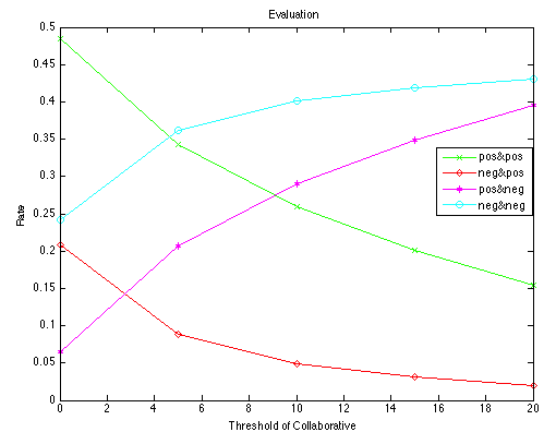
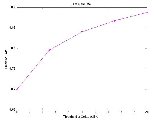
Figure 5: The evaluation at different thresholds

The figure at the left hand side shows the four different criteria value when we choose different thresholds. Here we are trying to maximize the value obtained by the green line divided by the red line, which equals to maximize the precision rate. As shown at the right hand side, the larger the threshold is, the better recommendation results we got, but meanwhile, we should notice that along with the increase of threshold, the lower the number of movies we recommend. Therefore, we have to balance between the number of movies recommended and the precision rate. Finally, we choose 10 as the threshold for collaborative part, and we guarantee a roughly 85% precision rate.

Demographical Filtering

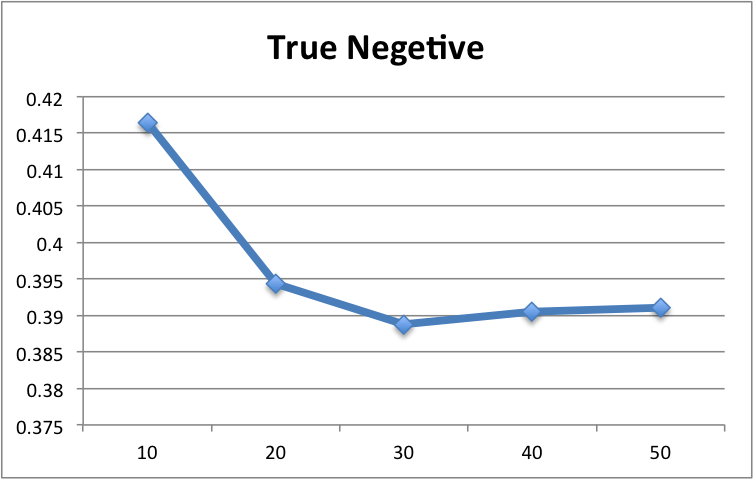
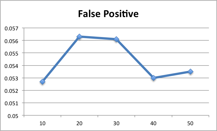
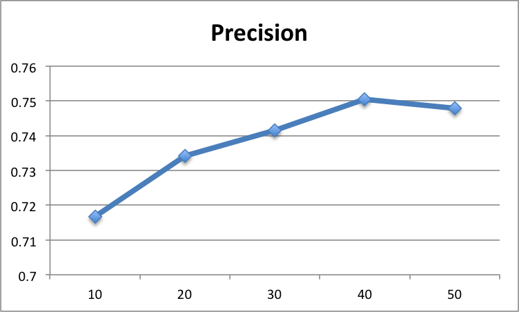
We test the performance of demographical filtering at different values of k. As mentioned before, we need to achieve the highest precision without lose of lower false positive. This avoids the algorithm to recommend a huge number of movies in order to achieve a better performance. Our experiment shows that when k=40, we get the best performance. The figures below demonstrate the result of our evaluation.

Figure 6: The evaluation at different k values

Content-based Filtering

The following graph shows the performance of using the three neural networks separately and the weighted prediction. We ran a program trying different weights on the training set and found that when w=[0.6,0.2,0.2] the system produces the best result.

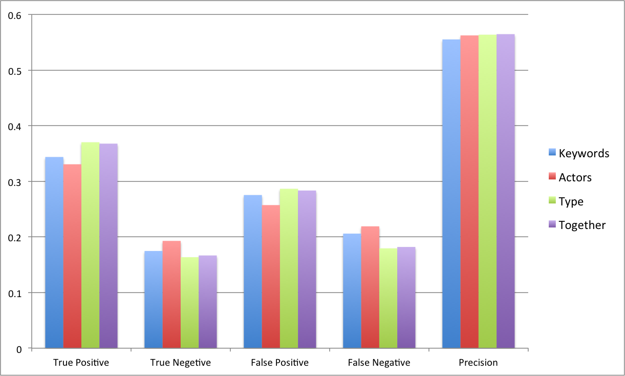
Figure 7: The evaluation of neural network

Hybrid Filtering

The graph shows the comparison of the result get from the three methods and the performance of the hybrid method. Because these three methods are using different scale to evaluate a movie, we adopted a voting strategy to produce the final prediction. We first consider those movies that are voted by all of the three methods. If we do not get enough movies to recommend, we further consider those that are voted by two of the methods. The purple is the result of using only those movies recommended by all of the three methods. We recommended about 900 movies out of 10,000 movies in the test set and 93 percent of them are actually liked by the users.

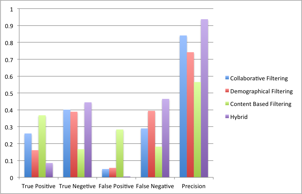
Figure 8: The evaluation of hybrid method