**Final project report**
(#) Juhyeon Kim (f006h11) and Jonathan Chiou (f003mcq)
(##) Motivational image
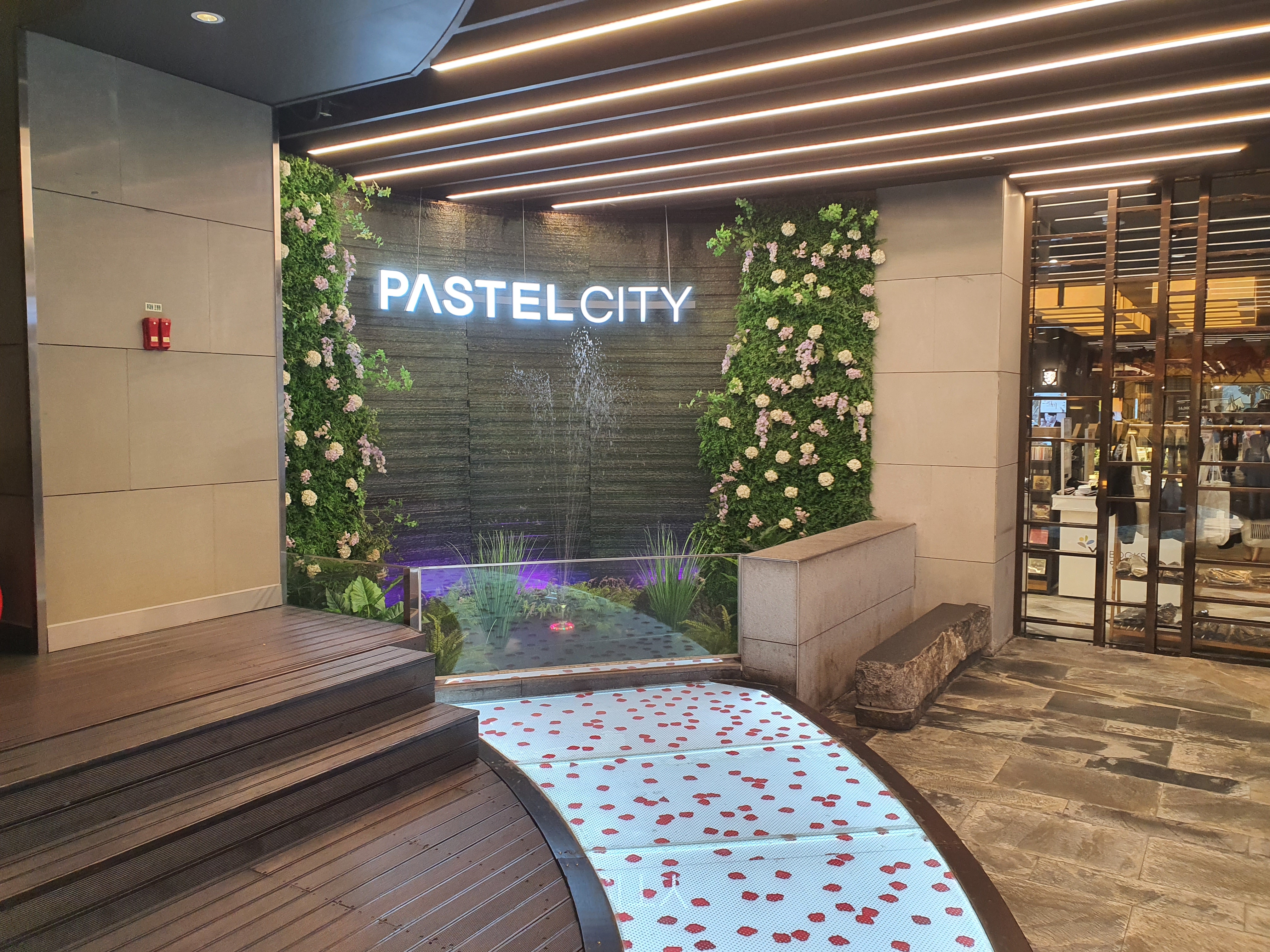
These are some photos I took which seem related to this year's theme. (Coloring outside the lines)
First photo is the entrance of the complex shopping mall named 'pastel city'.
This scene contains various colors with complex optical effects.
Water spreading out from the fountain, rainbow colored reflection and glassy floor, give an effect of colorfulness and dynamicness.
Second photo is a photo that I took at the exhibition whose theme was color and light.
There were many art works using lights with different colors.
They moved and sometimes overlapped over time, creating beautiful images.
The variety of colors wass not confined to a fixed screen, but had spread across the space over time, which I think fits into this year's theme.

Overall, what I want to show in the rendereed image is colorfulness and dynmicness.
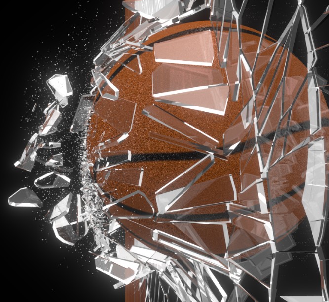
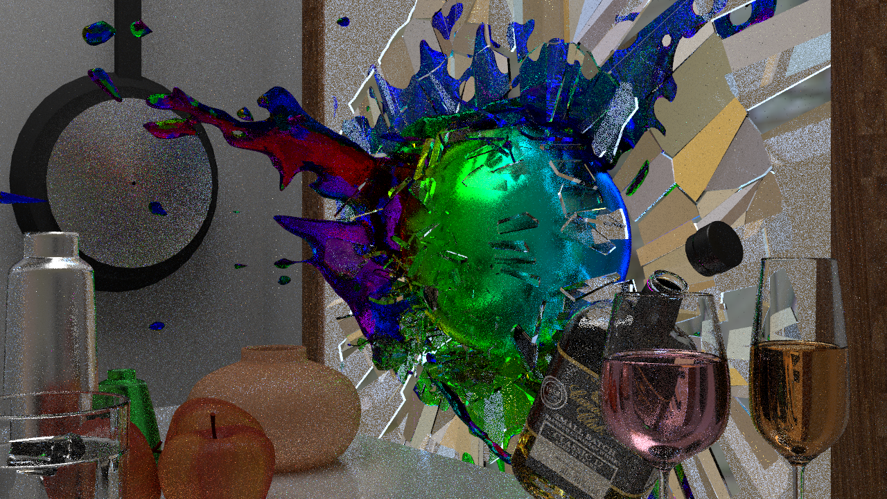
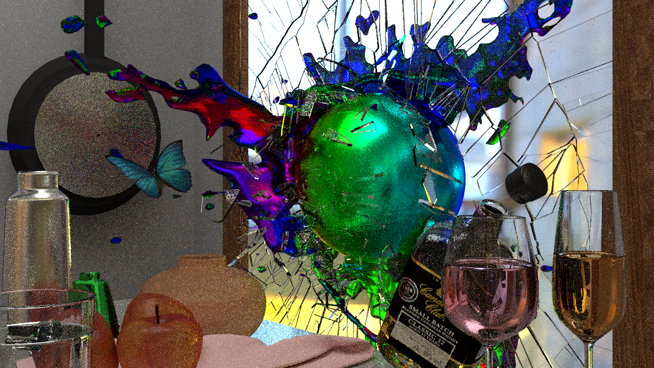
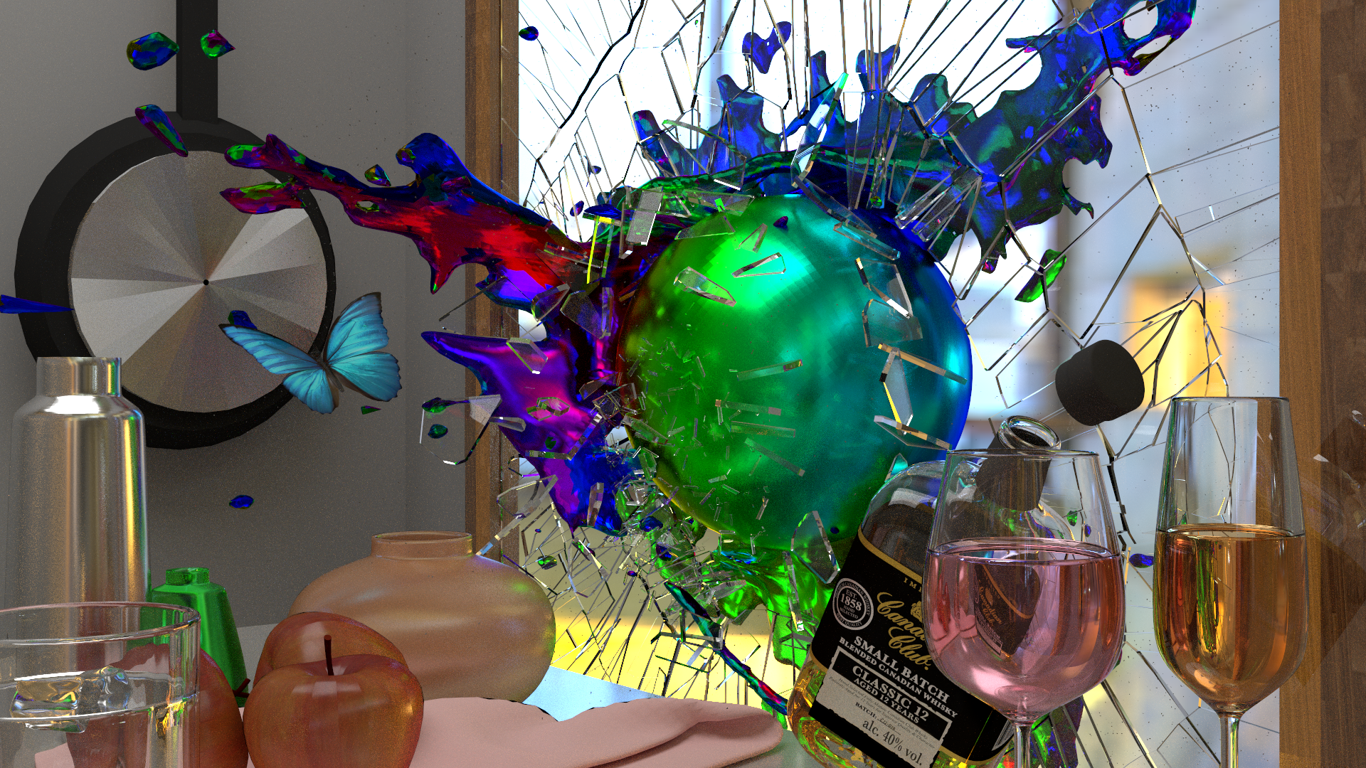
(##) Final Image Progress
I was motivated by this image in blender swap (https://www.blendswap.com/blend/15964).
I wanted to add some colors to so that image can both meet
colorfulness and dynamicness.
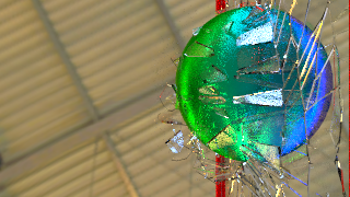
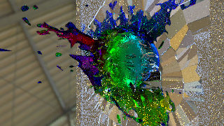
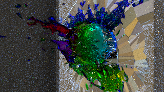
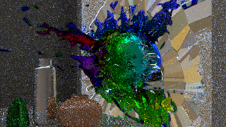
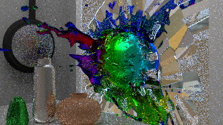
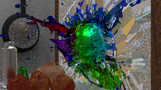
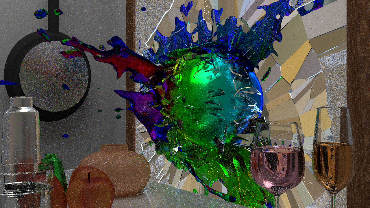
From now is the progress of the final image.
Starting from above blender file, I added more items to make the scene colorful.
Finally I added butterfly to the scene that really well represent
colorfulness and dynamicness.
(#) Implemented Features
From now, we will show our implemented features.
- 0. Environment map lighting
- 1. Material (physically based conductor, microfacet materials, anisotropic)
- 2. Multi threading
- 3. Photon mapping
- 4. Participating media
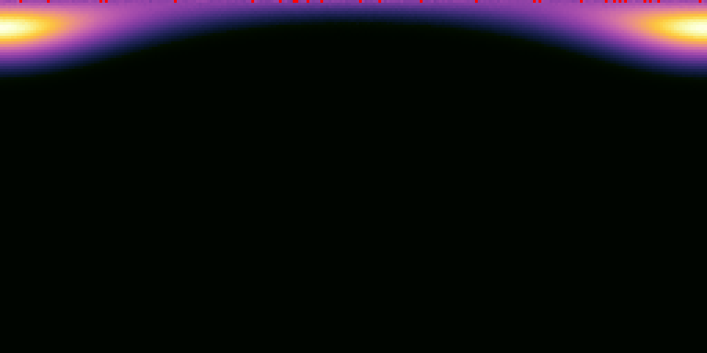
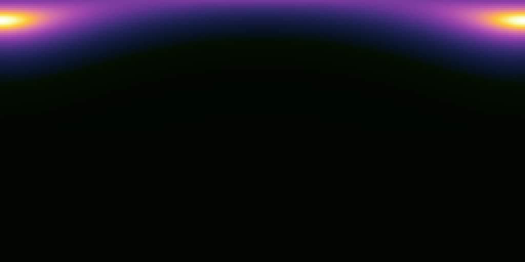
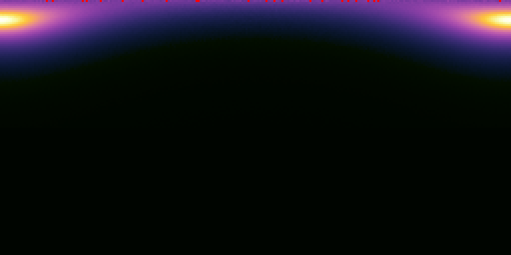
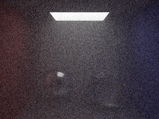
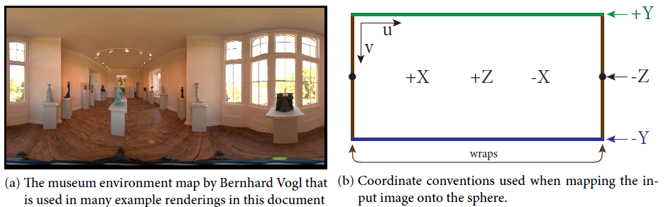
(#) 0. Environment Map Lighting
- code coordinate : src/scene.cpp, src/textures/envmap.cpp
We implemented environment lighting by changing background value from fixed color to texture.
I followed mitsuba coordinate system (y axis up).
The validation comes right after.
Because of time limit, I did not implement environment map importance sampling.
(#) 1. Material
We implemented new materials with physically based model.
Our overall implementation is largely inspired by mitsuba renderer [1] and paper of Walter et al [2].
Throughout material implementation, I compared GT image using Mitsuba renderer.
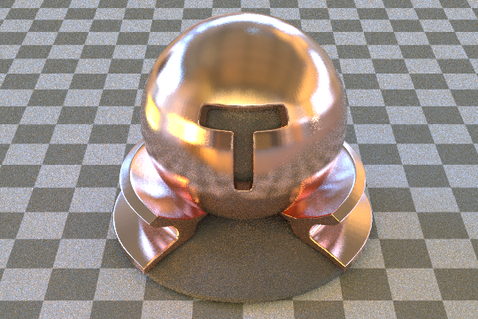
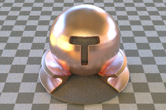
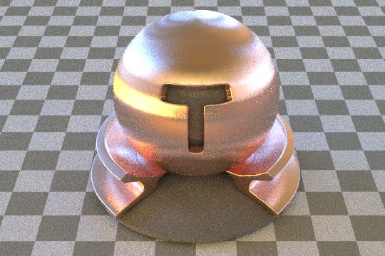
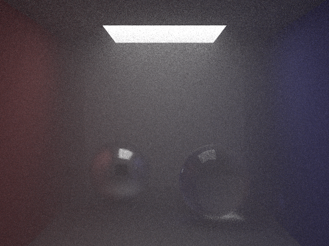
(##) (1) Conductor
- code coordinate : src/materials/conductor.cpp, include/fresnel.h
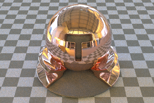
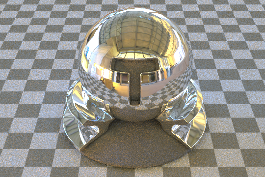
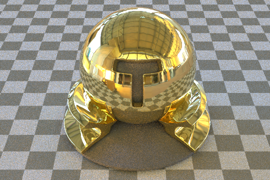
This is physically based model for metal-like material.
We use both real and imaginary component of IOR (eta-real, k-imaginary).
We assume no polarization, so average of s and p polarizations is used for fresnel term.
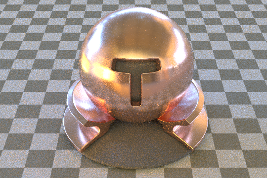
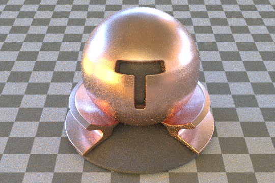
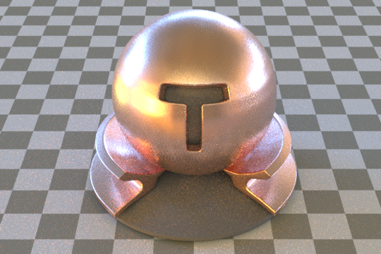
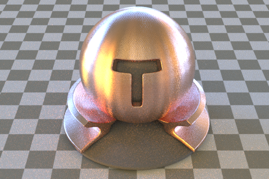
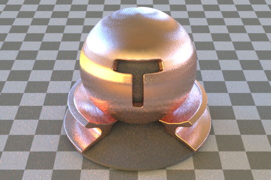
Here is results for three different conductor materials.
- Copper ("eta": [0.200438, 0.924033, 1.10221], "k": [3.91295, 2.45285, 2.14219])
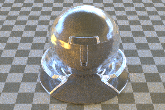
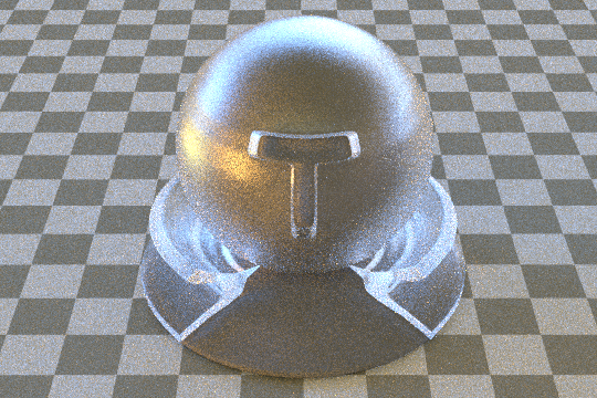
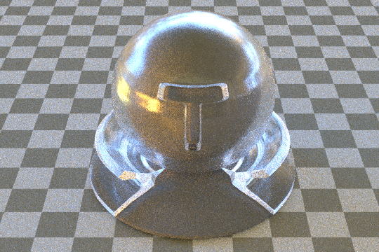
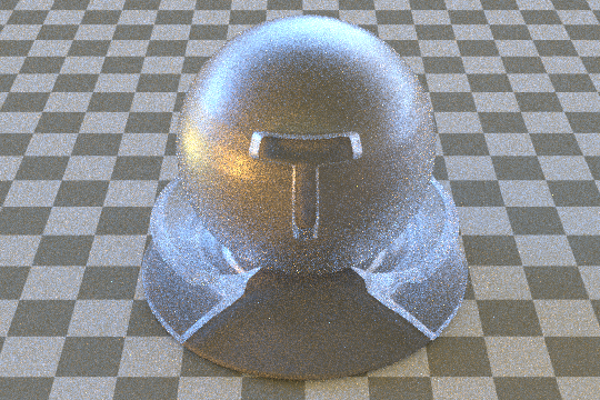
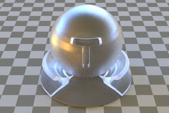
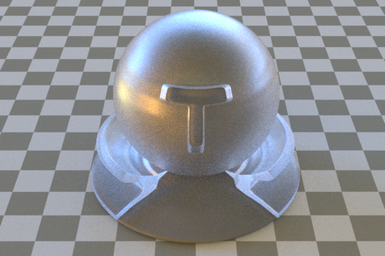
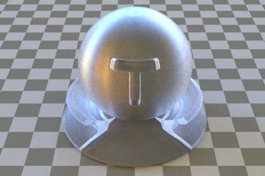
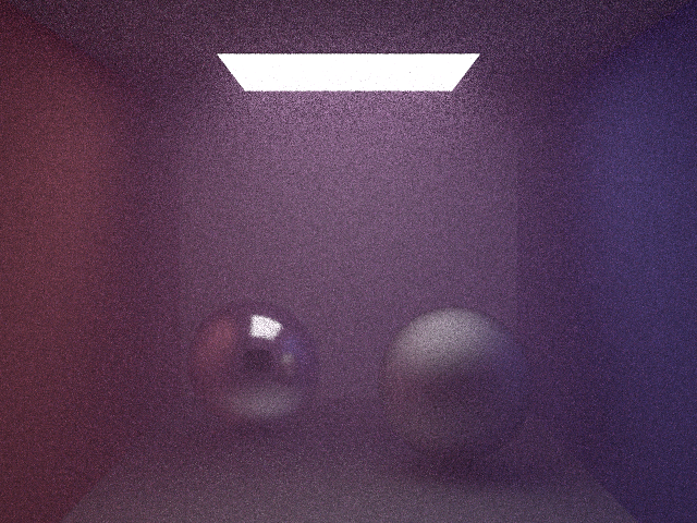
(##) (2) Rough conductor
- code coordinate : src/materials/roughconductor.cpp, include/fresnel.h, include/microfacet.h
For rough conductor, microfacet model is used.
I used assignment4's test code to validate sampling.
```
---------------------------------------------------------------------------
Running test for "beckmann-0.1"Evaluating analytic PDF │██████████████████████████████████████████████████████████████│ (1.434s)
Integral of PDF (should be close to 1): 0.9999999736066836
Generating 32768000 samples │██████████████████████████████████████████████████████████│ (4.064s)
100% of the scattered directions were valid (this should be close to 100%)
---------------------------------------------------------------------------
Running test for "beckmann-0.05"
Evaluating analytic PDF │████████████████████████████████████████████████████████████████████████████████████████████████████████│ (1.673s)
Integral of PDF (should be close to 1): 1.0000002522231541
Generating 32768000 samples │████████████████████████████████████████████████████████████████████████████████████████████████████│ (4.033s)
100% of the scattered directions were valid (this should be close to 100%)
---------------------------------------------------------------------------
Running test for "ggx-0.1"
Evaluating analytic PDF │████████████████████████████████████████████████████████████████████████████████████████████████████████│ (1.285s)
Integral of PDF (should be close to 1): 0.9894995740599357
Generating 32768000 samples │████████████████████████████████████████████████████████████████████████████████████████████████████│ (3.800s)
98% of the scattered directions were valid (this should be close to 100%)
---------------------------------------------------------------------------
Running test for "ggx-0.05"
Evaluating analytic PDF │████████████████████████████████████████████████████████████████████████████████████████████████████████│ (1.280s)
Integral of PDF (should be close to 1): 0.9973517841221807
Generating 32768000 samples │████████████████████████████████████████████████████████████████████████████████████████████████████│ (3.752s)
99% of the scattered directions were valid (this should be close to 100%)
Passed all 4/4 tests. Also examine the generated images.
PS C:\Users\cjdek\Desktop\projects\cs87-fall-2022-juhyeonkim95>
```
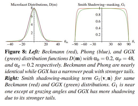
Here is pdf & sampled distribution results.
You can find a longer tail for GGX models which matches with Walter et al. [2].
- Roughness 0.05
- Roughness 0.1
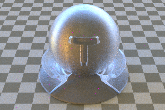
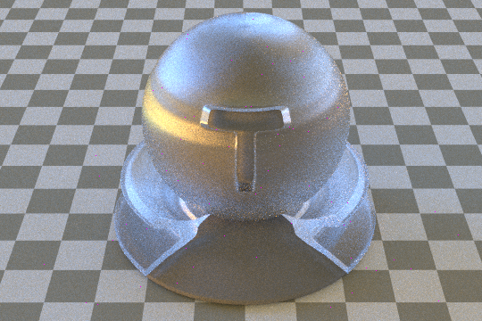
- Rendered Image
- Rendered Image vs GT
I also implemented anisotropic material.
Here is an example of anisotropic material.
I compared three images
- alpha = 0.05 (isotropic)
- alphaU = 0.3, alphaV = 0.05
- alphaU = 0.05, alphaV = 0.3
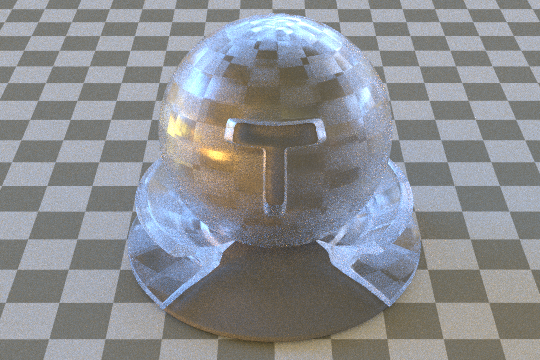
(##) (3) Rough Dielectric
- code coordinate : src/materials/roughdielectric.cpp, include/fresnel.h, include/microfacet.h
```
Contains alpha!
---------------------------------------------------------------------------
Running test for "dielectric beckmann-0.02"
Evaluating analytic PDF │██████████████████████████████████████████████████████████████████████████████████████████████████████████████████████████████████████████████████│ (2.262s)
Integral of PDF (should be close to 1): 1.0000058648977077
Generating 32768000 samples │██████████████████████████████████████████████████████████████████████████████████████████████████████████████████████████████████████████████│ (3.898s)
99% of the scattered directions were valid (this should be close to 100%)
Test failed: Some generated directions were below the hemisphere. You should check for this case and return false from sample instead.
Contains alpha!
---------------------------------------------------------------------------
Running test for "dielectric beckmann-0.1"
Evaluating analytic PDF │██████████████████████████████████████████████████████████████████████████████████████████████████████████████████████████████████████████████████│ (2.119s)
Integral of PDF (should be close to 1): 1.0000014196759281
Generating 32768000 samples │██████████████████████████████████████████████████████████████████████████████████████████████████████████████████████████████████████████████│ (4.005s)
99% of the scattered directions were valid (this should be close to 100%)
Test failed: Some generated directions were below the hemisphere. You should check for this case and return false from sample instead.
Contains alpha!
---------------------------------------------------------------------------
Running test for "dielectric ggx-0.02"
Evaluating analytic PDF │██████████████████████████████████████████████████████████████████████████████████████████████████████████████████████████████████████████████████│ (1.715s)
99% of the scattered directions were valid (this should be close to 100%)
Test failed: Some generated directions were below the hemisphere. You should check for this case and return false from sample instead.
Contains alpha!
---------------------------------------------------------------------------
Running test for "dielectric ggx-0.1"
Evaluating analytic PDF │██████████████████████████████████████████████████████████████████████████████████████████████████████████████████████████████████████████████████│ (1.723s)
Integral of PDF (should be close to 1): 0.9985430228865452
Generating 32768000 samples │██████████████████████████████████████████████████████████████████████████████████████████████████████████████████████████████████████████████│ (3.778s)
99% of the scattered directions were valid (this should be close to 100%)
Test failed: Some generated directions were below the hemisphere. You should check for this case and return false from sample instead.
Failed 4/4 tests. Also examine the generated images.
```
Note that pdf sample test fails because there is some directions below the hemisphere, which is not weird thing for dielectric material.
- Roughness 0.02
- Roughness 0.1
- Rendered Image
- Rendered Image vs GT
Similarly we can render anisotropic rough dielectric materials.
Finally, we can do some interesting thing using checkerboard alpha.
(##) (4) Others
I also implemented other materials (transparent / two sided), but it is not important, so I will omit them.
For transparent material, I added emission to reproduce bright butterfly.
(#) 2. Multi Threading
- code coordinate : src/scene.cpp
I also increased the rendering performance using multi threading.
Each ray sample from camera could be parallely simulated using multi threading.
Following is part of the code using multi-threading for rays.
```
// Create a worker per CPU thread
Pool *pool = pool_create(NANOTHREAD_AUTO);
Progress progress("Rendering", image.width() * image.height());
Task *task = drjit::parallel_for_async(
drjit::blocked_range(0, image.width() * image.height(), 1),
// Task callback function. Will be called with index = 0..999
[&](drjit::blocked_range range) {
for (uint32_t i = range.begin(); i != range.end(); ++i) {
int y = i / image.width();
int x = i % image.width();
Color3f color = Color3f(0.0f);
for(int n = 0; n < m_sampler->sample_count(); n++)
{
Vec2f offset = this->m_sampler->next2f();
auto ray = m_camera->generate_ray(Vec2f(x + offset.x, y + offset.y));
color += this->m_integrator->Li(*this, *this->m_sampler, ray);
}
color /= m_sampler->sample_count();
image(x, y) = color;
++progress;
}
},
{}, pool
);
// Synchronous interface: submit a task and wait for it to complete
task_wait(task);
```
Compared to not using multi-threading, there is a performance gain like following.
```
Will save rendered image to ".\scenes\multi-threading\jensen_box-w-multi-2022-11-19-14-18-44.png"
Rendering │█████████████████████████████████████████│ (20.581s)
Will save rendered image to ".\scenes\multi-threading\jensen_box-wo-multi-2022-11-19-14-19-21.png"
Rendering │█████████████████████████████████████████│ (38.732s)
```
While they give same results.
Using multithreading nearly doubles the performance.
I used per-pixel thread, but there can ba other variants such as per-block thead or per-sample thread.
(#) 3. Photon Mapping
- code coordinate : src/integrators/photon_mapper.cpp
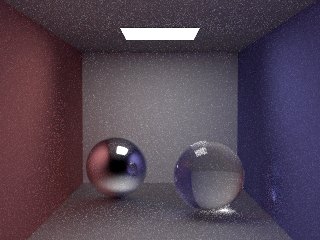
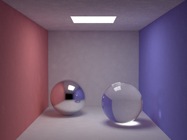
First, we implemented basic photon mapping.
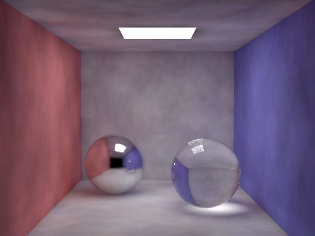
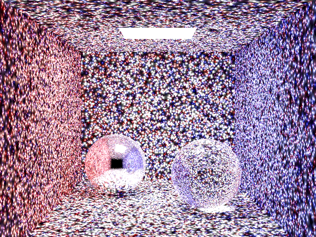
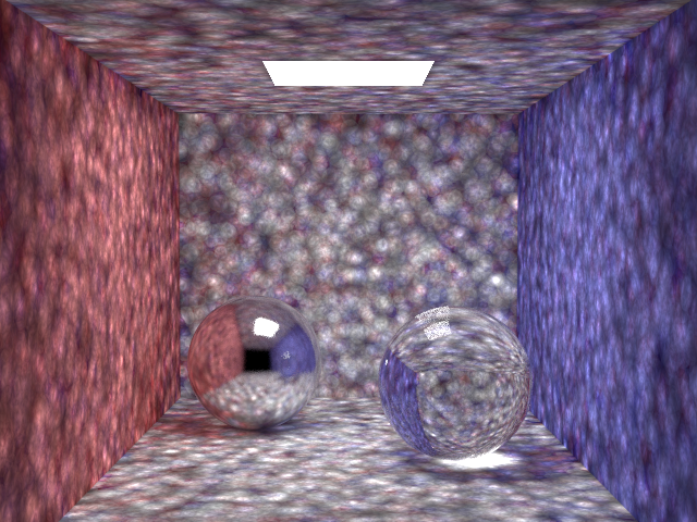
Following is demonstration of photon mapping using different number of photons or searching radius/number.
- Chaging number of photons
We implemented photon mapping with some improvements.
We build two photon maps, global photon map and caustics photon map.
Global photon map is a standart photon map while for caustics photon map, we store LS+D paths.
Illumination calculation is done in following ways.
First, trace path from camera until it hits the first non-specular surface.
Then we sum followings.
- Emission
- Direct illumination : use NEE
- Caustics : calculate from caustics photon map
- Indirect illumination : continue until next non-specular surface then calculate from global photon map
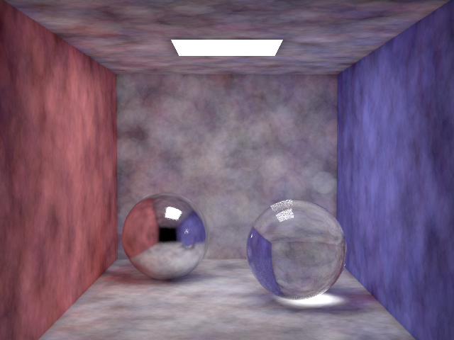
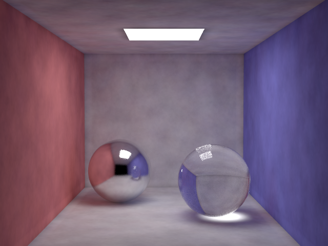
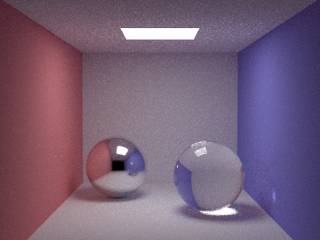
Here is the demonstration of improvement.
Compared to basic one, the improved one removes (1) over blurred caustics (2) splotches on the wall
and (3) bias near the edges.
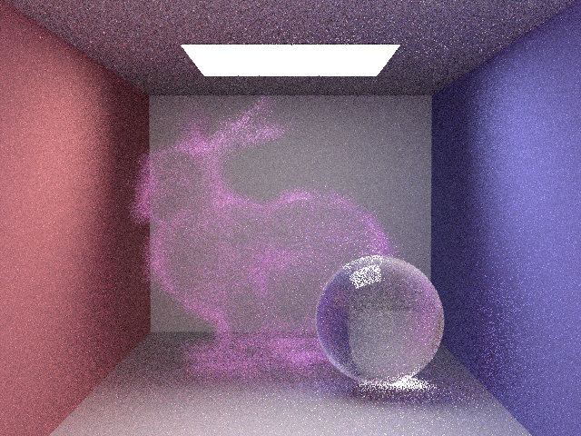
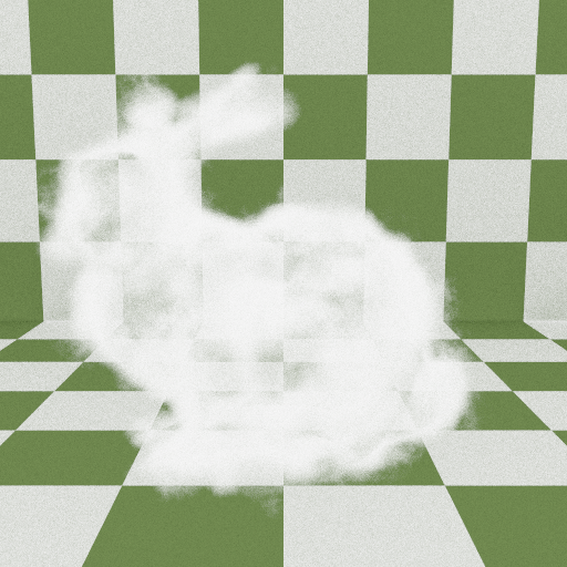
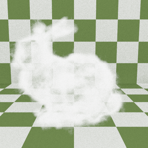
(#) Participating Media
Technical details of implementation:
- Supports both homogeneous and heterogeneous media
- Multiple Importance Sampled (MIS) distance using pdfs of each color channel
- Path tracing used both MIS and NEE, similar to assigment 5
- Interiors of specular objects are treated as a vacuum (no participating media) to avoid foggy glass
- Implemented isotropic phase function
Code coordinates:
- *Media:* `media/homogeneous.cpp: 50-80`, `media/nanovdb_medium.cpp: 125-175`
- *Integrators:* `integrator/volumetric_mats.cpp: 42-87`, `integrator/volumetric_mis.cpp: 49-110`
- *Materials:* `materials/isotropic.cpp: 55-92`
Validation tests are collected in the following three sections.
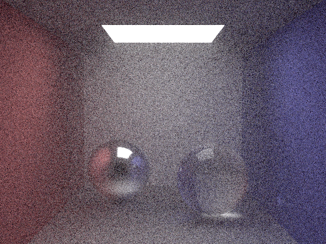
(##) Participating media: Homogeneous volumes
Some of the below test scenes will compare:
- an integrator that samples just materials (mats)
- an integrator that samples materials and lights (mis)
Test scene with infinite area light:
Test scene with a small quad light:
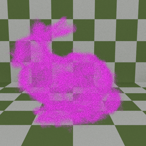
Test scene with colored medium:
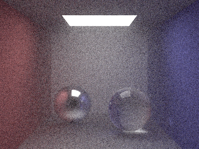
(##) 4. Participating media with Heterogeneous volumes
Test scene with infinite area light:
Test scene with a small quad light:
Test scene with colored medium:
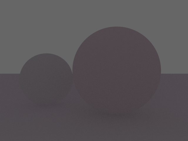
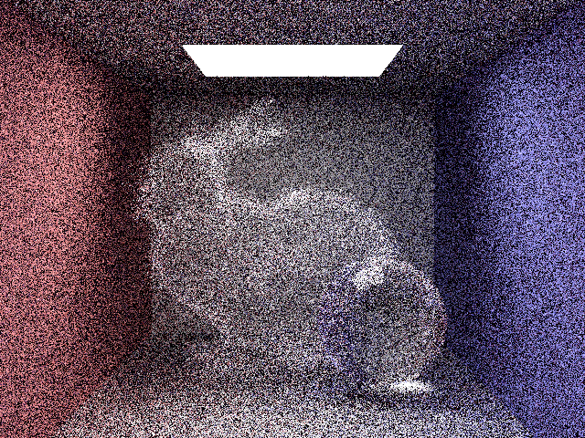
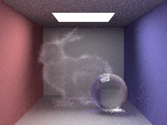
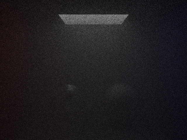
(##) Participating media: Challenges
We initially only had a materials-sampling integrator, which performed poorly in dim light settings.
Test case with dim lights:
Before handling interiors of specular objects, glass was foggy.
Test case with glass:
(##) What is used for final image
What is implemented and used
- Environment map lighting
- Microfacet materials
- Anisotropic materials
- Path tracer MIS with improvements (russian roulette, multi threading)
- Transparent material with emission (butterfly wing)
What is implemented but not used
- Photon mapping : because there are so may dielectric things in the scene, we found that photon mapping is not that effective.
- Participating media : we wanted to add volumetric things aroung butterfly, but because of time limit, we couldn't.
What is used but not implemented
- Fluid simulation : used fixed object
- Fracture simulation : used blender simulation
(##) Division of labor
0 ~ 3 : Juhyeon Kim
4 : Jonathan Chiou
- 0. Environment map lighting
- 1. Material (physically based conductor, microfacet materials, anisotropic)
- 2. Multi threading
- 3. Photon mapping
- 4. Participating media
Making scene / finding resources / running code : Juhyeon Kim
(##) Reference
[1] Jakob, Wenzel. "Mitsuba renderer." (2010): 9.
[2] Walter, Bruce, et al. "Microfacet models for refraction through rough surfaces." Proceedings of the 18th Eurographics conference on Rendering Techniques. 2007.
(#) Thank you!
 The validation comes right after.
Because of time limit, I did not implement environment map importance sampling.
(#) 1. Material
We implemented new materials with physically based model.
Our overall implementation is largely inspired by mitsuba renderer [1] and paper of Walter et al [2].
Throughout material implementation, I compared GT image using Mitsuba renderer.
(##) (1) Conductor
- code coordinate : src/materials/conductor.cpp, include/fresnel.h
This is physically based model for metal-like material.
We use both real and imaginary component of IOR (eta-real, k-imaginary).
We assume no polarization, so average of s and p polarizations is used for fresnel term.
Here is results for three different conductor materials.
- Copper ("eta": [0.200438, 0.924033, 1.10221], "k": [3.91295, 2.45285, 2.14219])
The validation comes right after.
Because of time limit, I did not implement environment map importance sampling.
(#) 1. Material
We implemented new materials with physically based model.
Our overall implementation is largely inspired by mitsuba renderer [1] and paper of Walter et al [2].
Throughout material implementation, I compared GT image using Mitsuba renderer.
(##) (1) Conductor
- code coordinate : src/materials/conductor.cpp, include/fresnel.h
This is physically based model for metal-like material.
We use both real and imaginary component of IOR (eta-real, k-imaginary).
We assume no polarization, so average of s and p polarizations is used for fresnel term.
Here is results for three different conductor materials.
- Copper ("eta": [0.200438, 0.924033, 1.10221], "k": [3.91295, 2.45285, 2.14219])
 - Roughness 0.05