**Rendering Algorithms (COSC87/287): Final project**
Varun Malladi (F003WYQ), Michelle Chen (F003KP4)
(#) Motivational image and theme
The theme of "coloring outside the lines" presented an opportunity for us to contend with race and colorism.
Where "the lines" become the boundaries on normativity, the act of "coloring outside" tranlates to existing outside those prescriptions —
specifically, existing within skin darker than the prescribed, pale ideal.
We were motivated by known biases in rendering and other graphical fields (i.e. the synonymity of "human skin" with "white skin")
to develop photorealistic algorithms with melanin-rich skin as the focus and not the edge case.
An additional layer to our interpretation of the theme emerged through fluorescent body paint.
Because fluorescent materials absorb UV light, and trend toward highly irregular spectral distributions,
and because body painting practices have largely Indigenous and/or non-Western origins,
the combination of the two introduces further nuance to "coloring outside the lines."
In this domain, what is traditionally non-white and non-Western intermixes with what literally falls outside the normal,
visible spectrum of light.
(#) Features: Point breakdown & distribution of labor
* Fluorescent materials (8 pts.): Varun
* Subsurface scattering (8 pts.): Michelle
(#) Part 1: Fluorescent materials
(##) Spectral rendering
**Relevant files**:
* `include/darts/spectrum.h`
* `src/spectrum.cpp`
* `src/spectrum_tests.cpp`
**What we did**:
* implemented a `SampledSpectrum` class similar to the one in the PBR book, but not an exact copy, and using local structures like `Vec3f`
* created a wavelength-to-RGB method
* used Monte-Carlo integration on the spectral rendering equation (1)
Fluorescent interactions are wavelength dependent, and so the first step in supporting this
feature was implementing spectral rendering, which performs calculations on energy levels
of specific wavelengths rather than RGB values. In practice, this means reworking all
instances of `Color3f` in our code.
There was a lot of infrastructure that needed to be put in place, and much of this was
based off PBRv3's implementation of spectral rendering. Among these features were:
* representations of spectral power distributions (SPDs) with support for arithmetic
* ability to load SPD sample data into the above representation
* conversion to/from RGB color
With these in place, we could pass around a `SampledSpectrum` class everywhere there
used to be a `Color3f`, and simply convert from/to RGB when parsing the scene and
writing the image file, respectively. This corresponds to handling every wavelength
sample (later we will do something different). Because there are multiple possible
SPDs for a given RGB color (metamers), we should expect the colors in a scene rendered
with spectral rendering to be different than scenes rendering with RGB rendering.
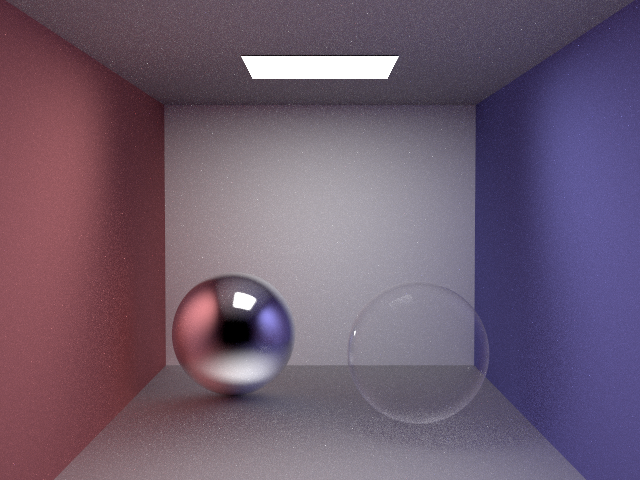
Nonetheless, we verified at this point that the basic features were the same:
(both images above used material sampling exclusively).
The following is the result of
our wavelength-to-RGB method, with varying wavelengths from 280-780 nm:
Handling all sampled wavelengths at each ray intersection was not attractive when thinking
about wavelength-dependent interactions. Consider the following version of the
rendering equation which includes wavelengths:
\begin{equation}
L_o(x,\omega_o,\lambda_o) = L_e(x,\omega_o,\lambda_o) + \int_\Omega\int_\Lambda L_i(x,\omega_i,\lambda_i)f_r(\omega_i,\lambda_i,x,\lambda_o,\omega_o)\cdot\cos\theta_i\ d\lambda_i d\omega_i
\end{equation}
The approach in PBRT with doing arithmetic on `SampledSpectrum` rather than `Color3f` is
not completely accurate, and only works if there is no wavelength-dependent interaction.
To account for such interactions, we should handle one wavelength per path. Without
certain optimizations such as reusing paths, this is considerably slower.
Spectral rendering can be thought of as another dimension of the
rendering equation integral, and we opted to use Monte Carlo integration and sample a
certain number of wavelengths from the visible spectrum.
(##) Fluorescent materials
**Relevant files**:
* `src/materials/diffuse_fluorescent.cpp`
* `src/materials/uv_light.cpp`
* `src/integrator/fluorescent_mats.cpp`
* `src/integrator/fluorescent_mis.cpp`
**What we did**:
* created normalization and sampling methods for SPDs in `SampledSpectrum`
* created a `DiffuseFluorescent` class for diffuse fluorescent materials
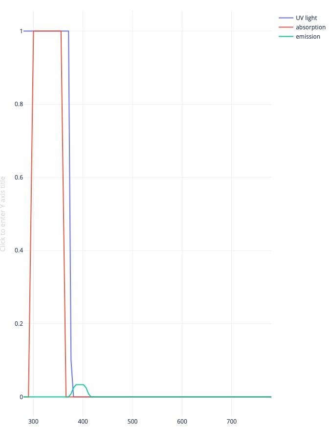
The key concept is that fluorescent materials absorb light at one wavelength and re-emit
it at another.
We can simulate this with a camera ray by first sampling a random wavelength at the
very beginning, then seeing if it intersects a surface with this material and lies within
that surface's emission spectrum, and sampling a new wavelength from the absorption
spectrum. The probability of a fluorescent interaction is 0 for camera-ray wavelengths
outside the emission spectrum's support, and dependent on the emission SPD values for
wavelengths within it.
To support such sampling, we needed to support general sampling for piecewise linear
functions. In the below pair of images, the points in the left one which have nonzero
height defined the piecewise graph we are sampling from, and the right image shows our
samples with random heights to improve visibility:
With this in hand, we can sample from (normalized) SPDs. A helper function was created to
normalize SPDs, since absorption spectra data in particular is often not normalized.
From there, we created the `FluorescentMats` and `FluorescentMIS` integrators using the approach
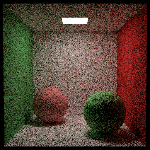
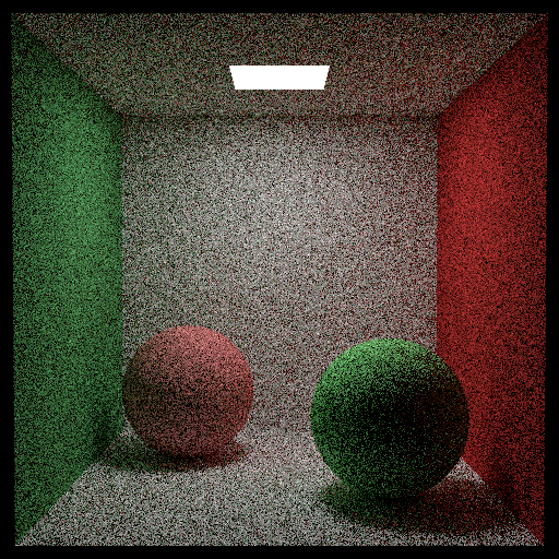
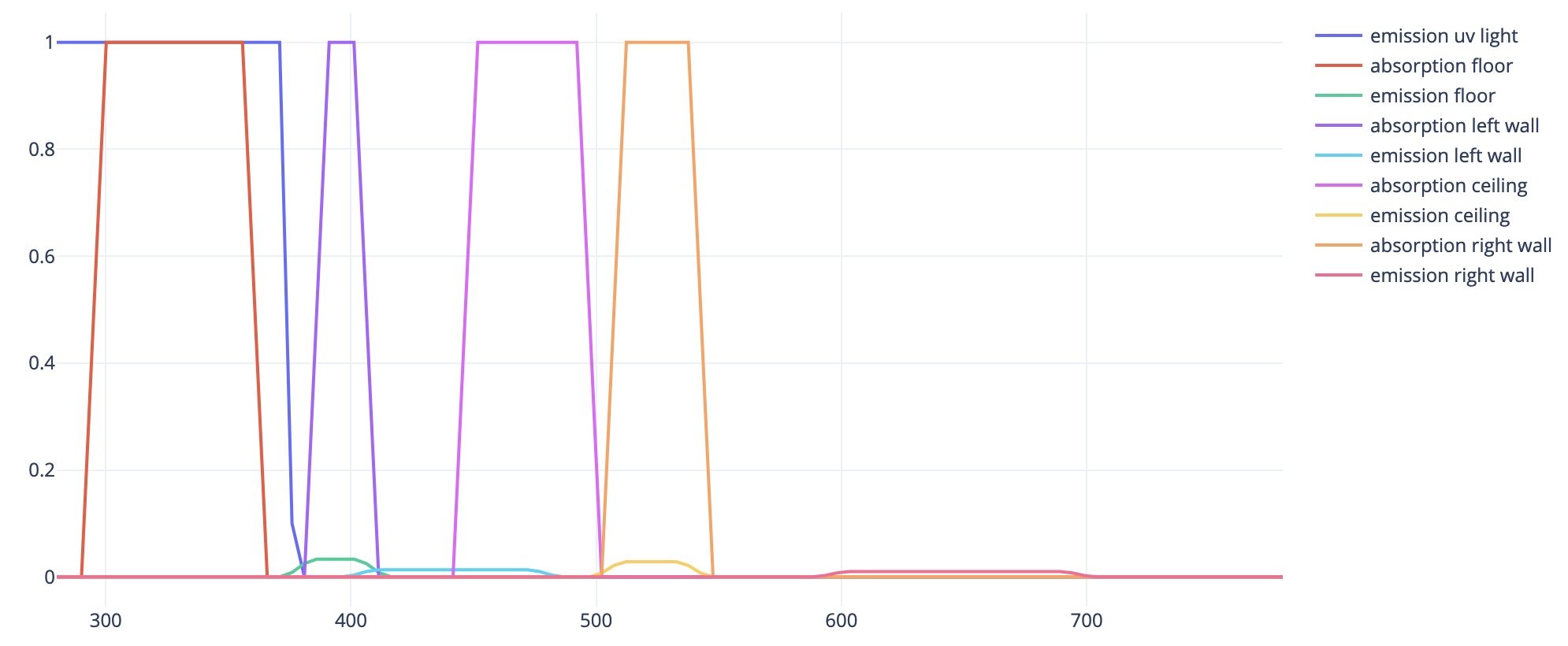
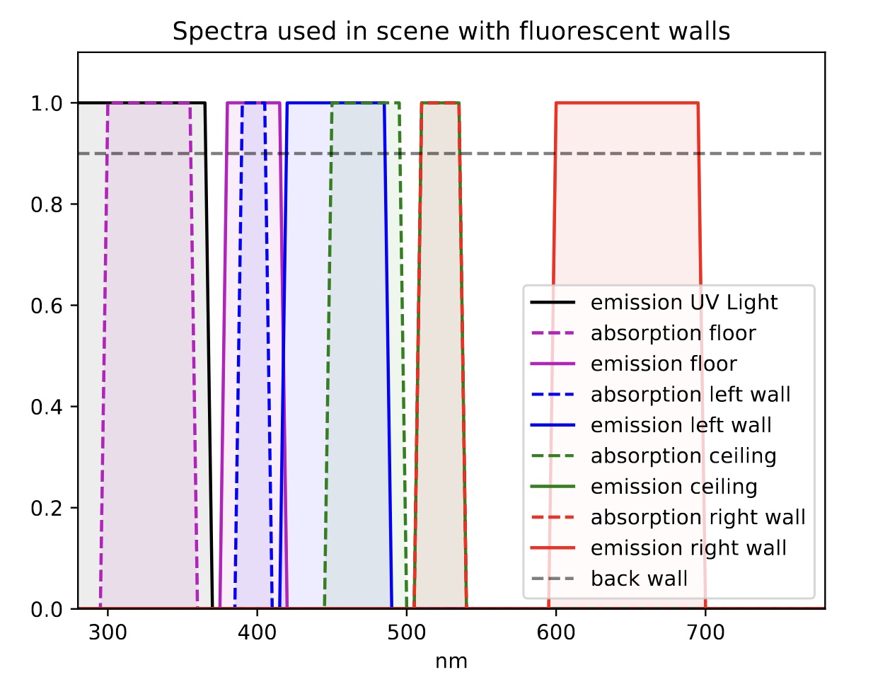
in (1) and (2). For validation, we mocked the example scene from (2):
(our emission spectra are normalized)
The point of this scene is the overlapping absorption/emission spectra. The floor will be the only
one with direct illumination, the left wall will get lit up by the floor, the ceiling will get lit
up by the left wall, and the left wall will get lit up with the ceiling. The back wall will get
lit up by all the walls and ceiling.
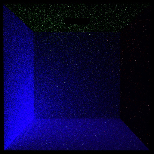
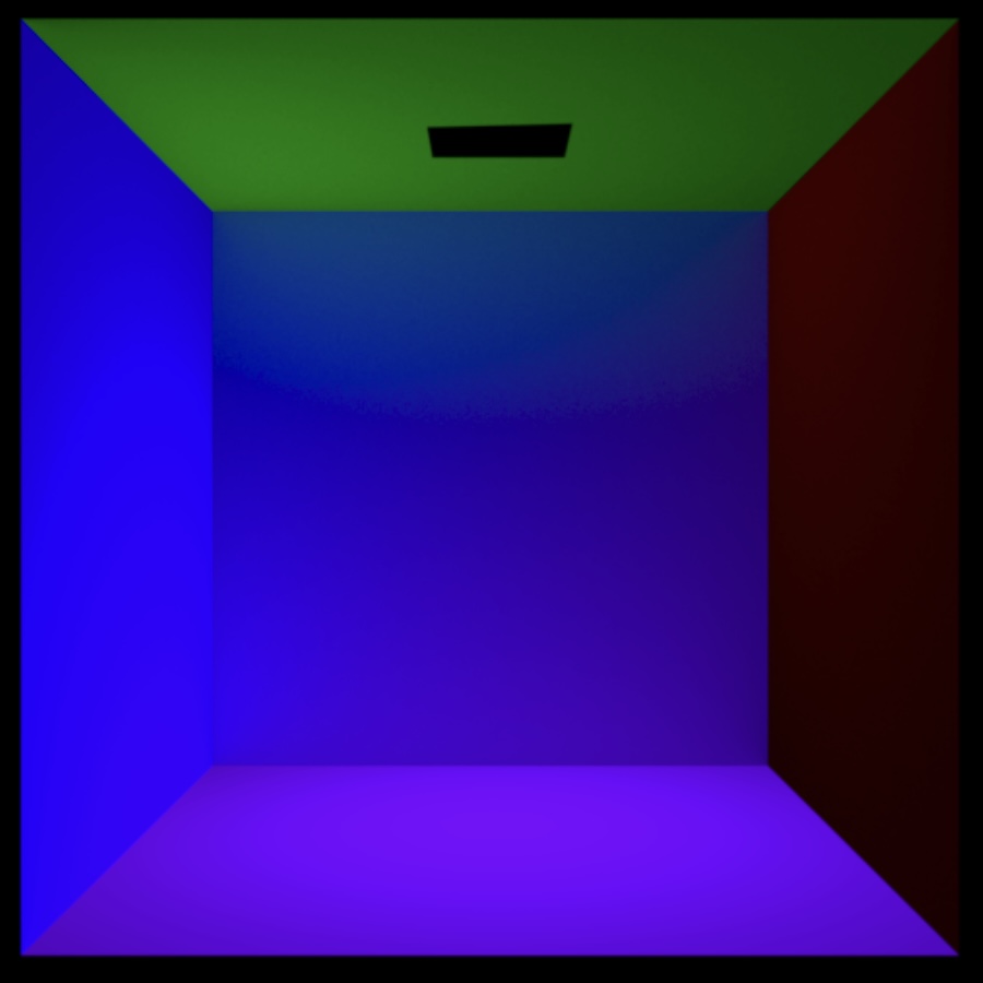
Our version had its exposure boosted and used a 100 sample, 10 wavelength-sample MIS render.
The reference used a 10,000 sample bidirectional, full wavelength-range render. We did not know
the colors used in the reference scene, only the spectra, and used our best guess. We did not
pursue higher-sample validation since this render already took several hours, and we believe it
demonstrated the correct behavior already. In particular, the floor is the clearest, followed by
the left wall, ceiling, and right wall because of the overlapping nature of the spectra.
(##) References
1. "A Simple Diffuse Fluorescent BBRRDF Model", Jung et al.
2. "Fluorescence in Bidirectional Rendering", Jung
(#) Part 2: Subsurface scattering
(##) Homogeneous Henyey-Greenstein (HG) Medium
**Relevant files:**
* `include/darts/medium.h` (NOTE: We overhauled the provided Medium base class.)
* `src/media/homogeneous_HG.cpp`
(Many existing base classes — Integrator, Parser, Surface, Mesh, Triangle, Quad, and Sphere — were also modified to be compatible with this implementation.)
The **Henyey-Greenstein phase function**, which we use to represent scattering in the homogeneous medium, takes three input parameters:
1. An asymmetry parameter, `g`, which controls the distribution of scattered light between forward-scattering and back-scattering. In other words, it is the average value of the product of two things: a) the phase function being approximated, and b) the cosine of the angle between and '.
2. The (total) extinction coefficient, `sigma_t`, which determines how frequently volumetric scattering within the medium occurs.
3. The scattering coefficient, `sigma_s`, which determines how much light scatters at each scattering incident.
Adjusting these three volumetric scattering parameters allowed us to represent different participating media. (A vacuum is `g=0.0`, `sigma_t=0.0`, and `sigma_s=0.0`.)
(##) Volumetric Path Tracing
**Relevant files:**
* `src/integrators/path_tracer_volumetric.cpp` (basic)
* `src/integrators/path_tracer_volumetric_mis.cpp` (MIS)
We also implemented volumetric path tracing to render these participating media.
(##) Testing features with renders
**Jensen box**
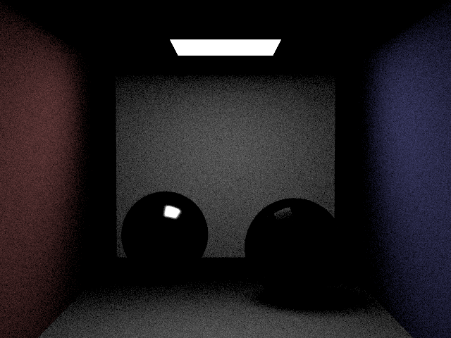
1. Box in a vacuum
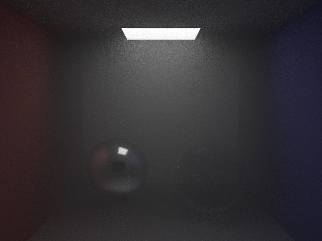
To first validate the functionality of the homogeneous medium representation and the volumetric path tracer (as well as the changes made to scene parsing/base classes), we reconstructed the Jensen scene: preserving all of its original geometry (the two spheres in the box, with an overhead quad light) and respective materials, BUT assigning two vacuums as participating media to each surface, one for each side. The desired outcome would be a scene that resembled the original, pre-participating-media scene.
The scene we created was `jensen_box_vol.json`. We tried to render it with the basic volumetric path tracing integrator. This yielded the following result, which was obviously incorrect:
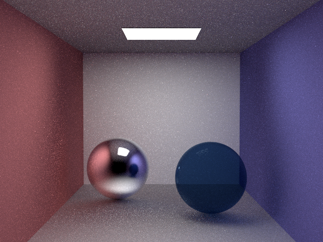
This motivated us to extend the volumetric path tracer to include multiple importance sampling, which yielded significantly more accurate results (scene: `jensen_box_vol_mis.json`):
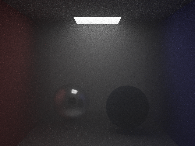
2. Box enshrouded in fog
To test the functionality of the scattering parameters g, sigma_t, and sigma_s, we rendered a foggy Jensen box. The only change we made was replacing every ‘vacuum’ participating media (for both sides of each surface) with a ‘fog’ participating media, where g = 0, sigma_t = 1.0, and sigma_s = 0.2.
**Head in a box**
1. Representing (skin) colors of dielectric boundaries through the scattering albedo property
Because we were interested in developing rendering techniques that did not privilege accuracy for lighter skin, we rendered a variety of skin tones, and tested each on up to six different participating-media representations.
To represent skin color …
In our JSON scene: We specified a scattering albedo property, `scatter_albedo`, for the dielectric boundary that corresponds to the outermost layer of skin.
In code (`src/materials/dielectric.cpp`): We created an absorption member variable that takes on a value through the constructor — which parses `scatter_albedo` and performs the following calculation: `absorption = 1.f - j.value(“scatter_albedo”, Vec3f(0.f))`.
To test for correctness, we revisited the Jensen box-in-a-vacuum scene (as well as the Jensen box-in-heavy-fog scene), and moved on when we achieved satisfactory results with the dielectric right sphere — to which we assigned a blue color.
2. Representing subsurface light transport in skin
Per Professor Jarosz’s recommendation, we sought to represent subsurface light transport in human skin through an exterior dielectric boundary containing an interior homogeneous medium.
*Background*
Real human skin behaves extremely complexly.
There are “multiple layers within the skin” — these are the living epidermis, papillary dermis, upper blood net dermis, reticular dermis, deep blood net dermis, subcutaneous fat, and blood — and each of these layers “absorb[s] and scatter[s] light differently.”
While graphics researchers have modeled optical scattering in skin with as many as five separate layers (see the five-layer BioSpec model developed by Krishnaswamy & Baranoski 2004), the accuracy and efficiency of a two-layer representation has been established through numerous other models (i.e. Takatania & Graham 1979, van Gemert et al. 1989, Spott et al. 1997, Tsumura et al. 2003, Donner & Jensen 2006). The lattermost listed paper states that “a closer analysis of the properties of different layers of skin” demonstrates “little variation in their optical properties,” affirming that “a two-layer separation into an epidermal and dermal layer is adequate.” Thus, our constraints in computation and time led us to informedly constrain ourselves to a two-layer representation of skin.
*Volumetric scattering parameters (g, sigma_t, sigma_s) for human skin*
Naito et al.’s 2014 publication, “Measurement of Scattering Phase Function of Human Skin,” represents skin as a homogeneous medium with “10.4 mm^-1 for the extinction coefficient,” “0.94 for the albedo,” and similarly “adopt[s] the Henyey-Greenstein (HG) function,” with an “asymmetry factor, g[,] of 0.9.”
We adopted this phase function with these parameters for our homogeneous skin medium.
*Testing with one-layer skin*
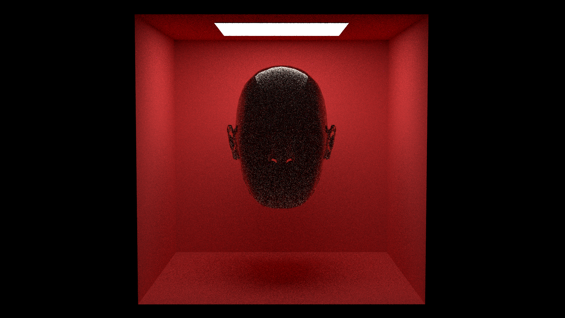
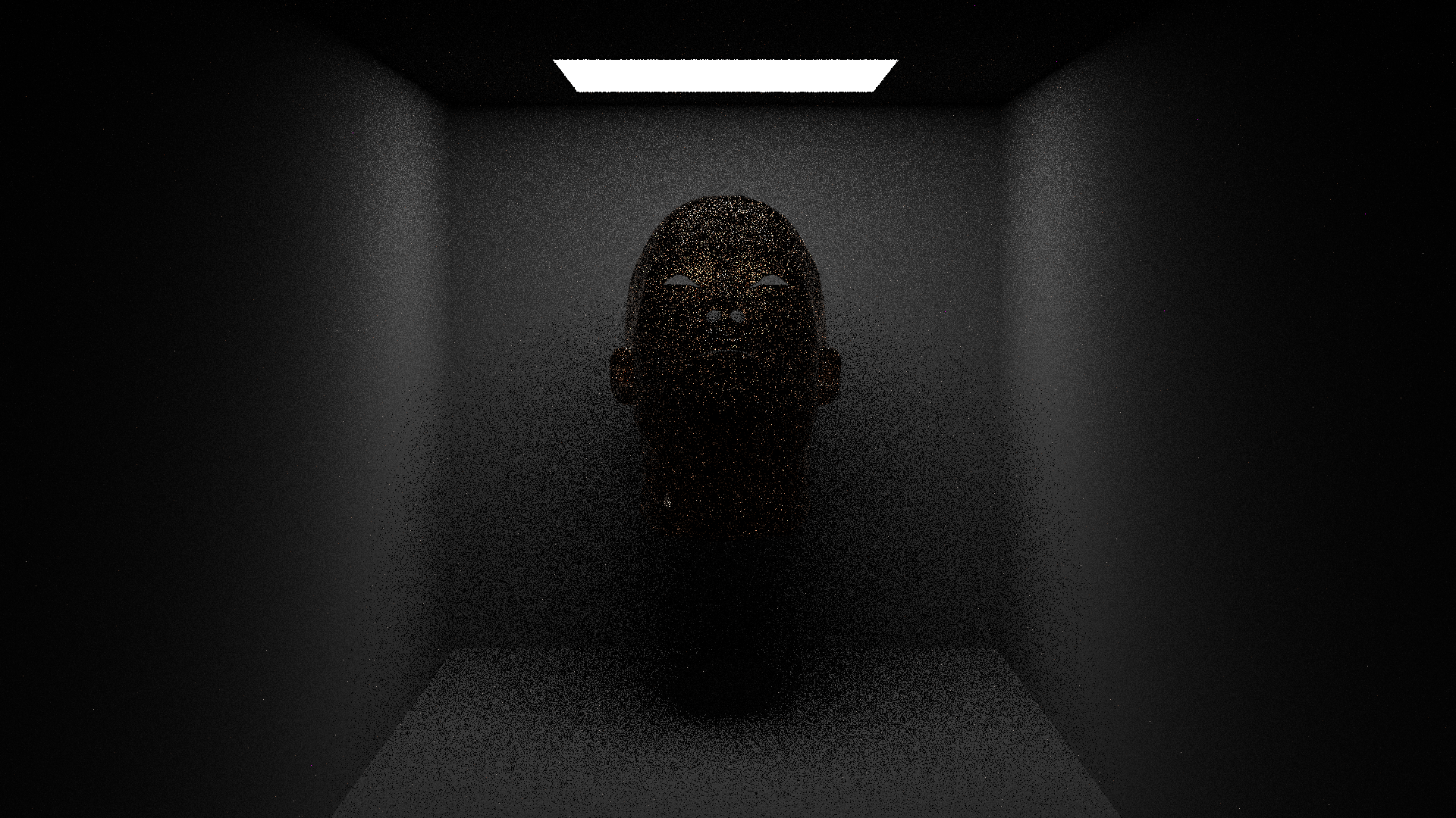
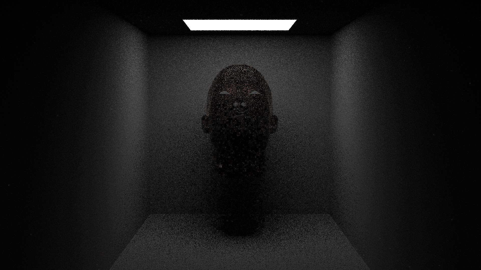
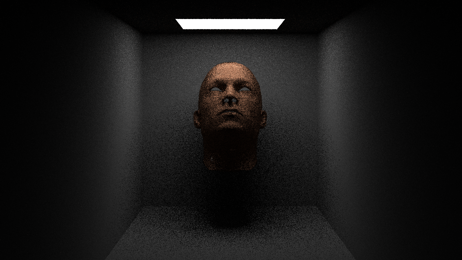
To evaluate the accuracy of our scattering parameters, we constructed a test scene with a one-layer representation of skin. We imported a human head mesh from [here](https://www.turbosquid.com/3d-models/soldier-head-3d-model-1765707) (with some adjustments made to it in Maya; namely, sealing the opening below the neck) into our scene; set its material to be dielectric, with an IOR of 1.5; and set its two media to be ‘vacuum’ and ‘skin,’ respectively.
While some subsurface light transport effects were visible at this stage — accumulating in thinner regions, such as the ears, as anticipated — the front of the face received too little light, and so accuracy was indeterminable.
We decided to tilt the head upward to the light for subsequent two-layer tests.
*Testing with two-layer skin*
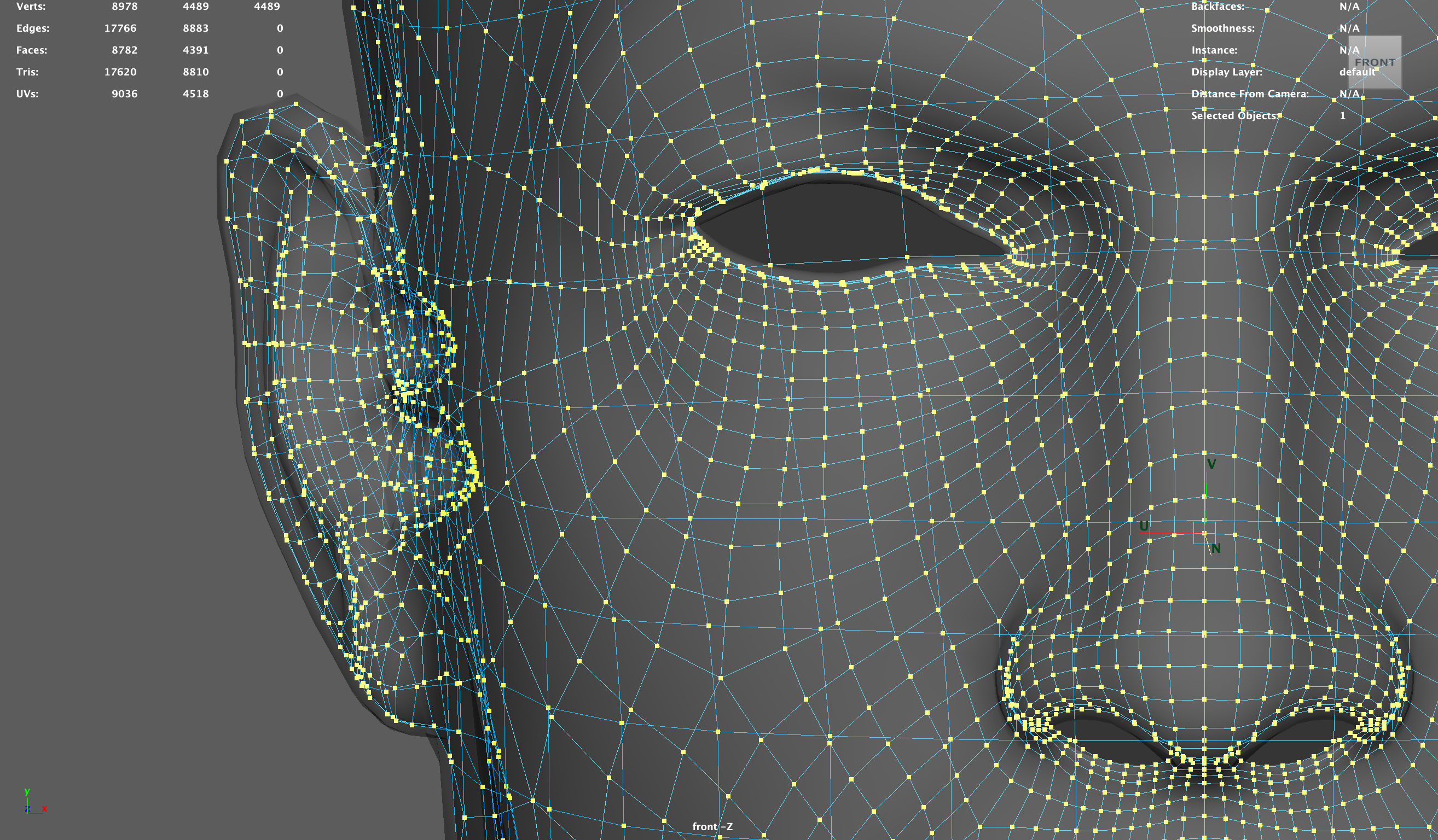
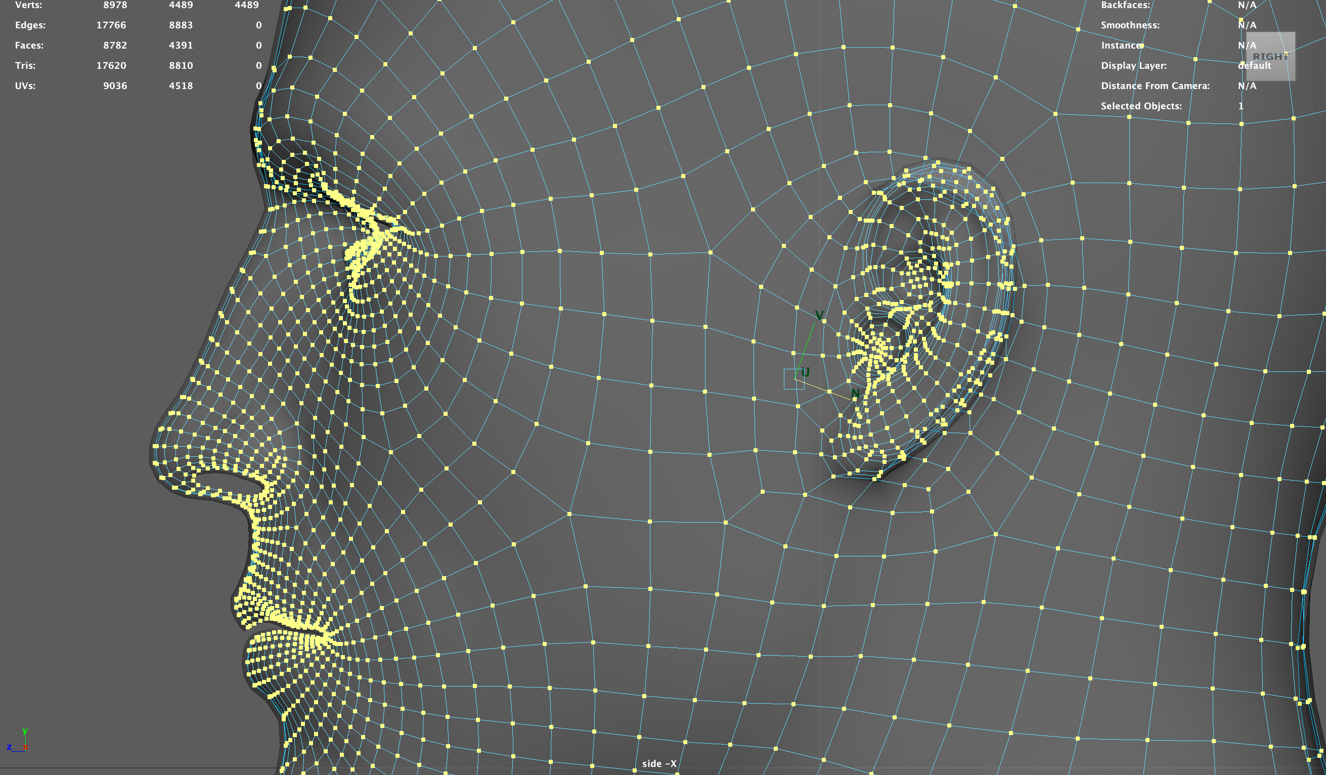
For our two-layer representation, we used two meshes: an “exterior” head mesh and an “interior” head mesh.
The exterior is the unaltered original, whereas the interior is a duplicate of the exterior, but downsized. This downsizing cannot be trivially performed through a simple rescaling of the object on its live axis. Doing so results in warping/deformation, as evinced here…
However, selecting all of the object’s vertices and scaling them down along the normal axis preserves an equidistant relationship between each vertex of the interior and its corresponding vertex on the exterior. This leads to nondeformed results — aforementioned equidistance then lends itself nicely to a sense of constant “skin depth.”
In our JSON scene, we assigned a dielectric material to the exterior head mesh, and a lambertian material to the interior head mesh. (Just as the color of the dielectric exterior is determined via `scatter_albedo`, the color of the lambertian interior is determined via the albedo.)
We then experimented with different configurations of participating media for both. To track how these configurations affected our test renders, and to increase ease of visual comparison, we named our scenes and files accordingly, with the following notation:
“VVVV” (vacuum-vacuum/vacuum-vacuum) configuration: The exterior and interior are each assigned both ‘vacuum’ media.
“VSSS” (vacuum-skin/skin-skin) configuration: The exterior is assigned the ‘vacuum’ medium and the ‘skin’ medium. The interior is assigned both ‘skin’ media.
“VVSS” (vacuum-vacuum/skin-skin) configuration: The exterior is assigned both ‘vacuum’ media. The interior is assigned both ‘skin’ media.
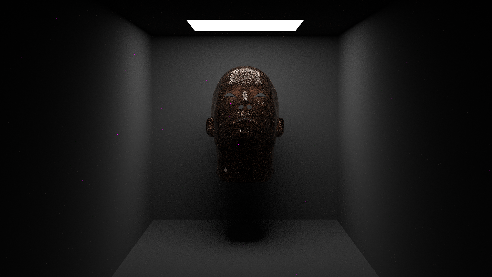
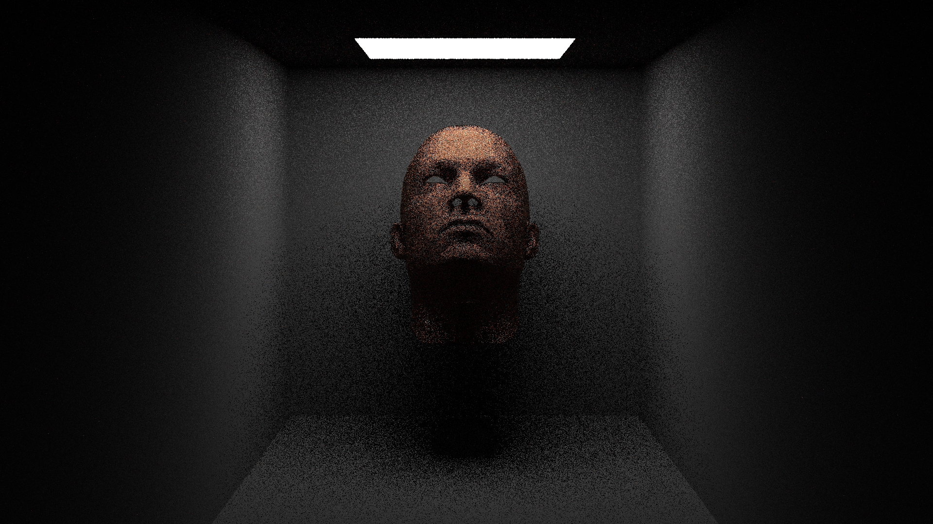
As a control, we tested “VVVV” — a configuration that places everything in a vacuum. Both skin tones came out extremely washed out and un-melanated. The renders (expectedly) took very little time to finish; 1 sample required approximately 1.5 minutes.
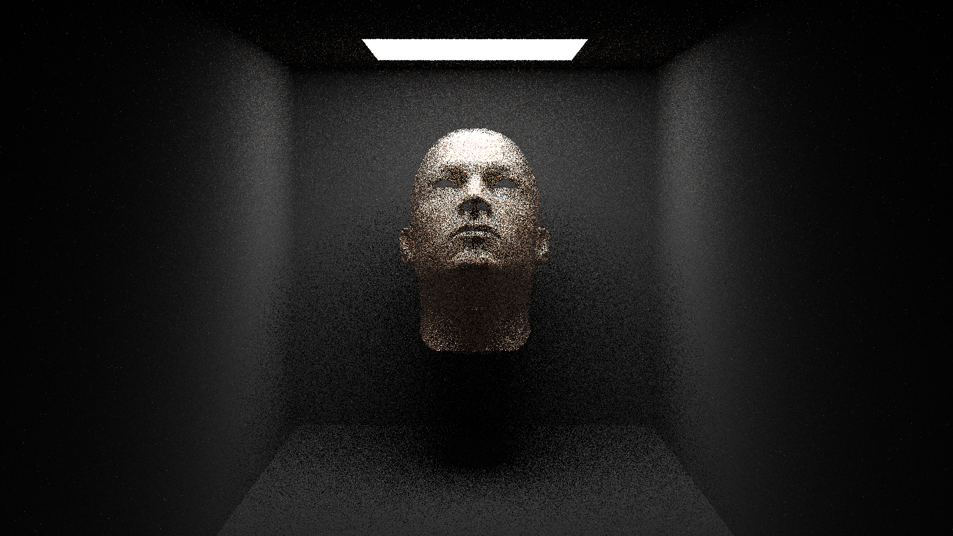
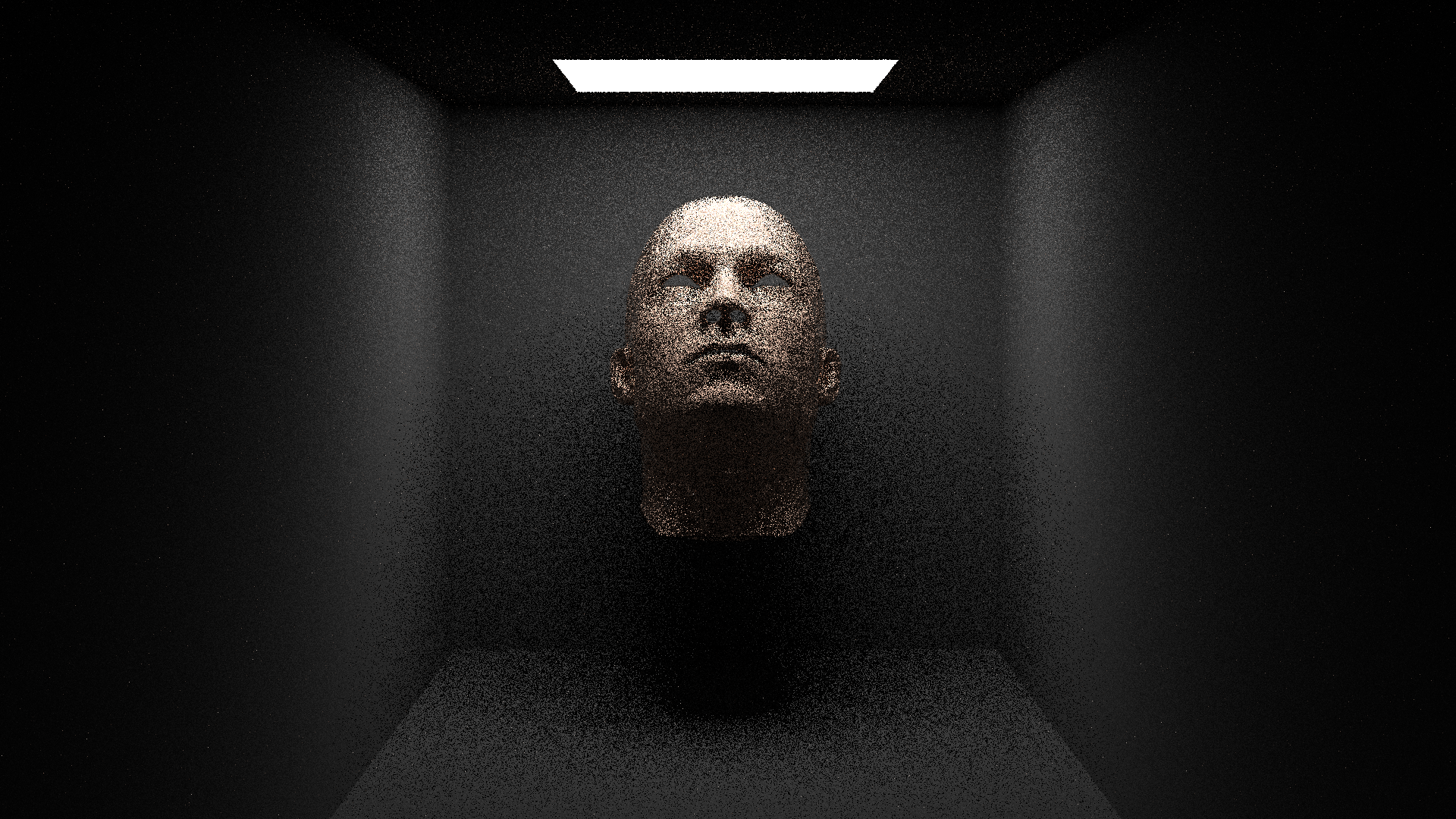
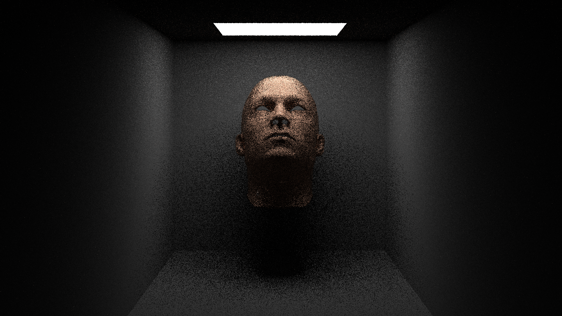
We then tested VSSS — adopting, essentially, the old configuration for the media of the exterior, but adding a pure-skin-media interior.
We found that, while the results represented significantly more accurate skin tones*, the volumetric scattering of the skin remained problematic. The skin took on a synthetic, wax-like appearance. There was an unrealistic glossiness that was especially noticeable in the lighting on the forehead and nose. Furthermore, the overall light distribution was flawed. The ‘depression’/groove on the innermost section above each eye, where the skin dips inward between the elevations of the brow and nose, should be darker than its surrounding regions. In VSSS renders, however, these regions were lighter.
*The skin tones were realistically human, but were darker than the specified albedo properties should have led them to be. We hypothesize that the darker tones comes not from a realistic representation of the provided parameters, but from higher noise (considering the significantly longer render-times from both VVVV and VVSS).
In terms of time, VSSS was notably more expensive than VVVV; 1 sample required approximately 9 minutes.
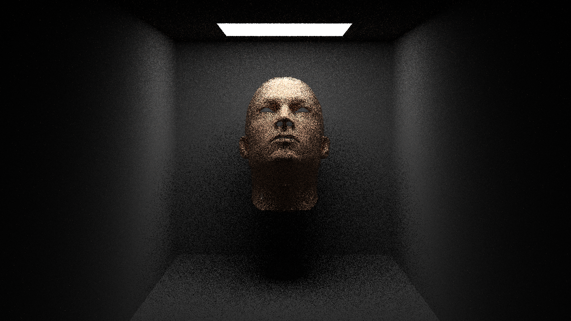
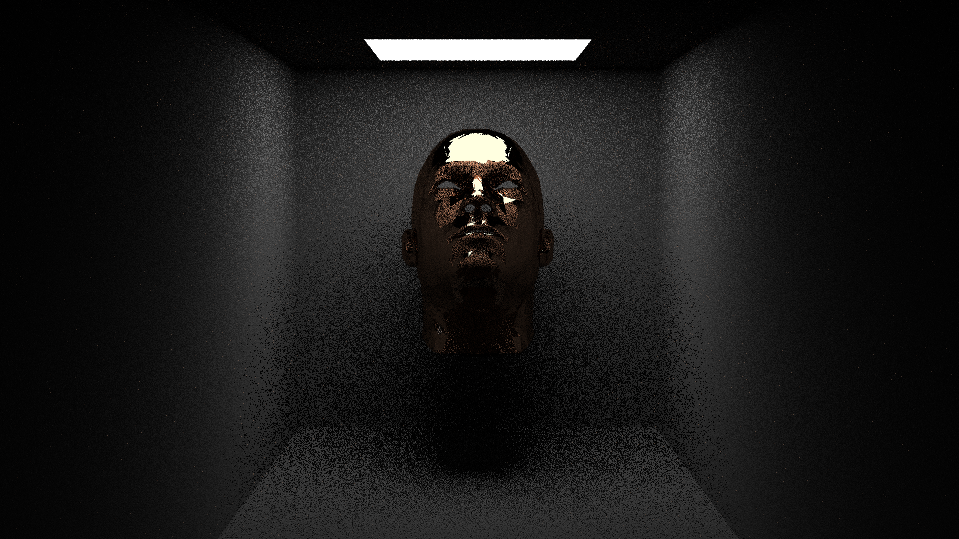
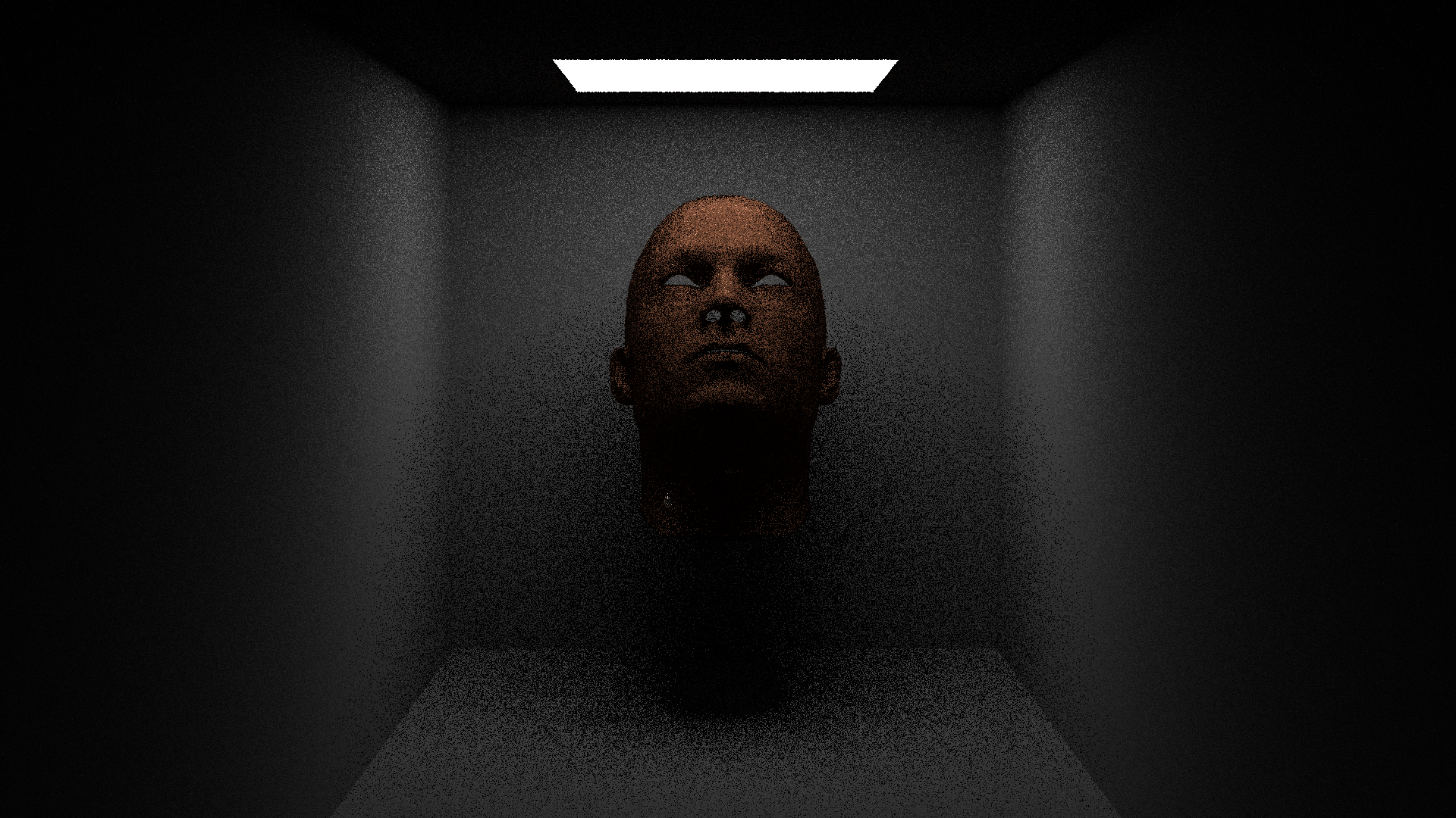
Finally, we tested VVSS. This returned the most accurate results among all configurations. The disappearance of the glossiness, as well as the realistic light distribution (note that the aforementioned inner-eye region is now correctly darker than its surrounding regions), led us to decide on this configuration for our final render. We thus tested it on a wider variety of skin tones, as well as a variety of reflective IORs, and found that an IOR of 1.1 appeared most qualitatively accurate (with an IOR of 1.3 a little too reflective, and an IOR of 0.75 far too unrealistic — almost cel-shader-esque in its outcome).
Skin tone 1:
Skin tone 2:
Skin tone 3 (IORs of 0.75, 1.1, 1.3):
Skin tone 4:
We ultimately decided to render skin tone 4 for our final.
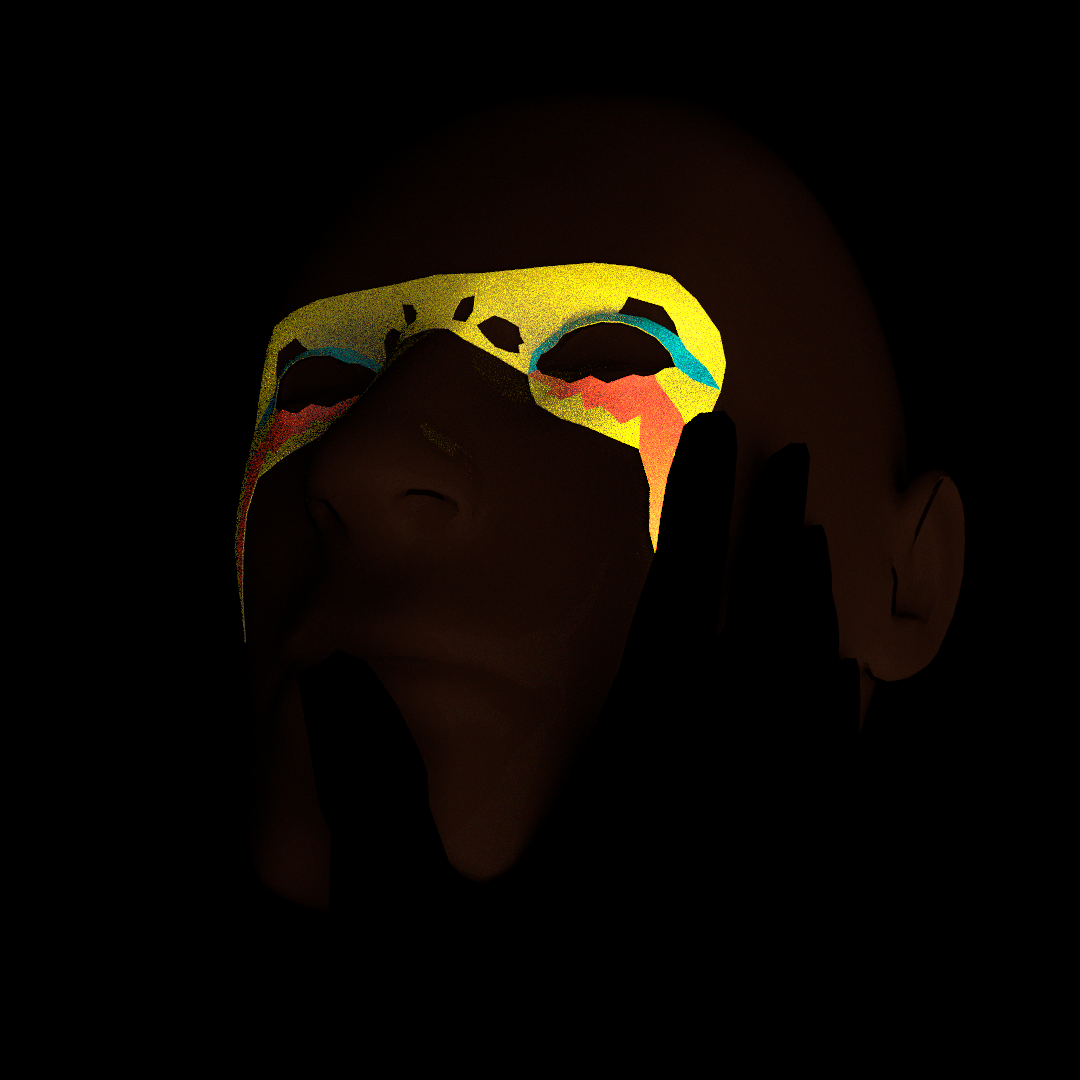
(#) Final render: Combining fluorescence with subsurface scattering
In rendering darker skin, we wanted to convey that the stories of people of
color are "outside" ones that are typically told.
The black hand represents the stories in our family that were never told, the disconnect
from family and family history. Nonetheless, the hand is actually emitting UV light. While
one can't see it directly, this hand lights up the face.