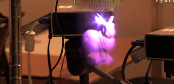
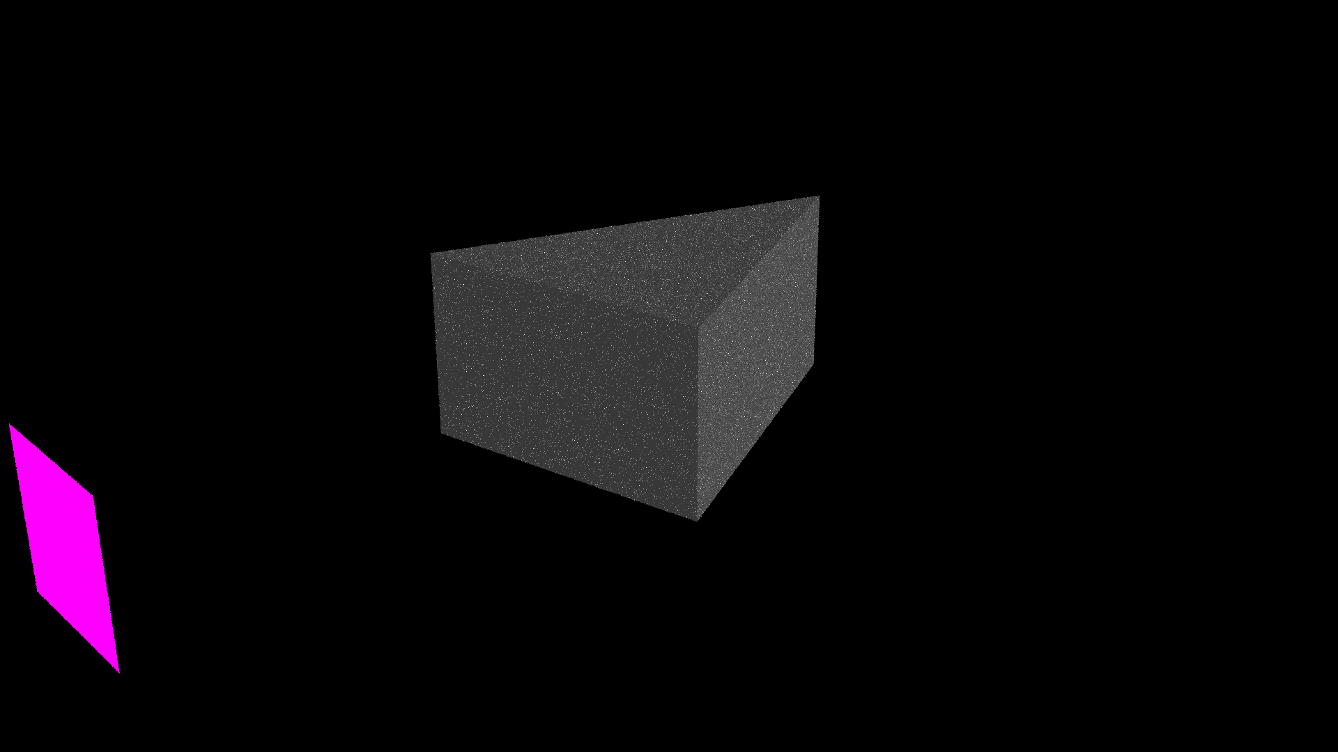
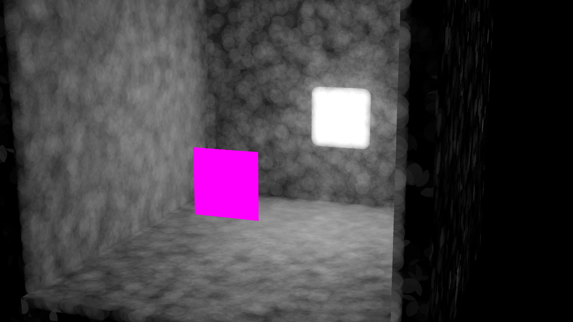
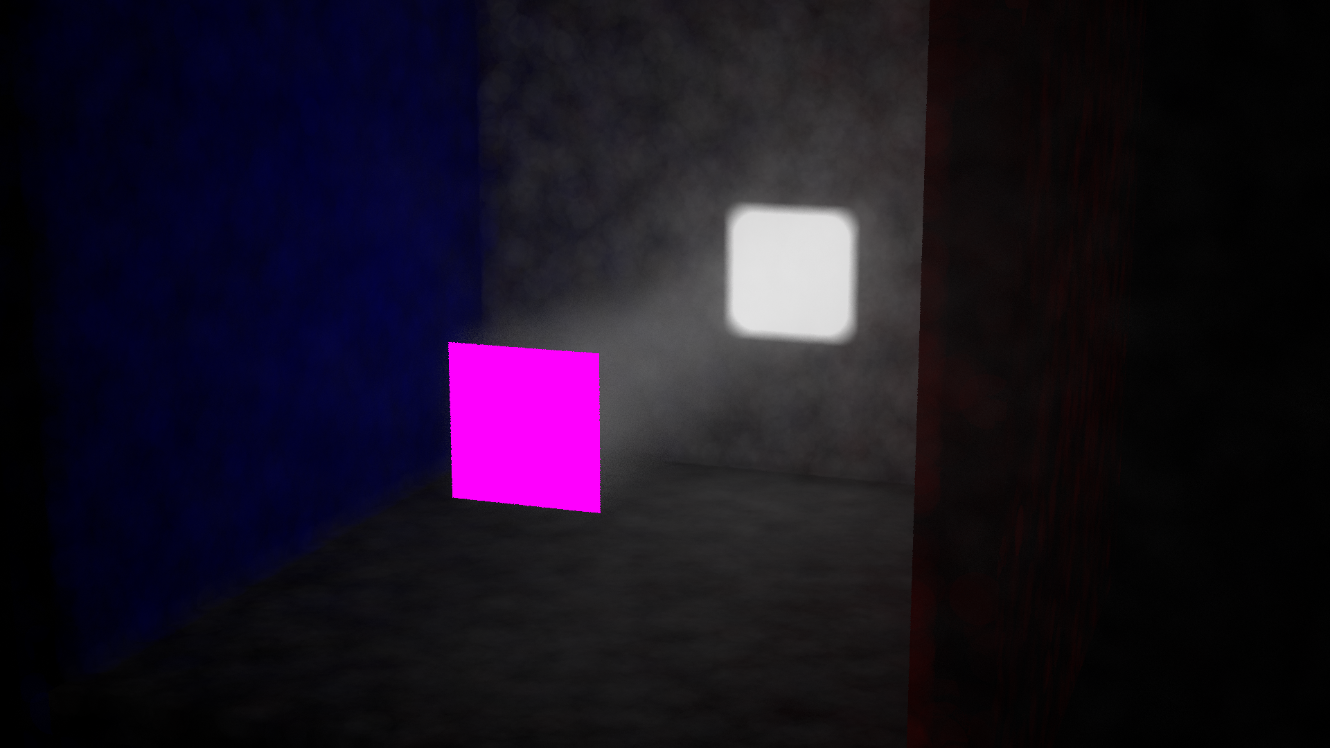
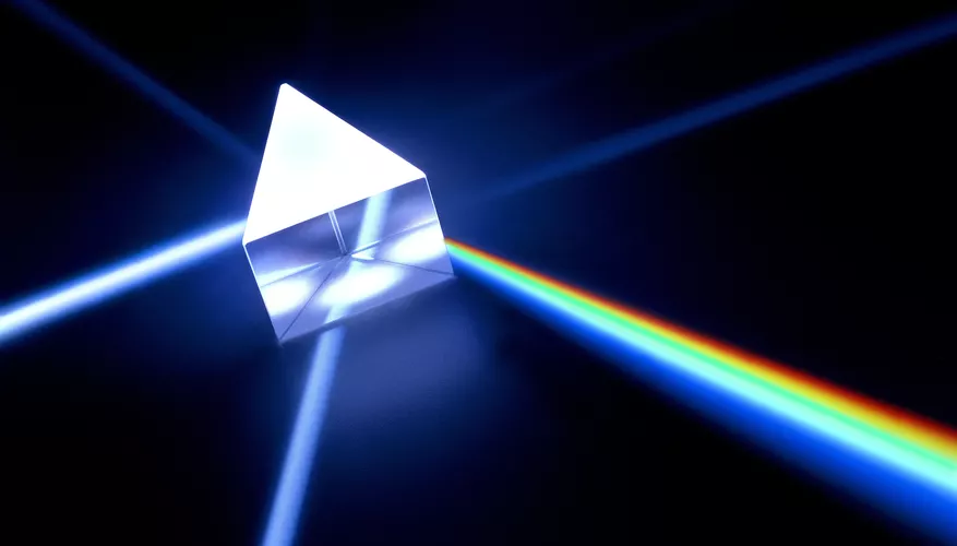
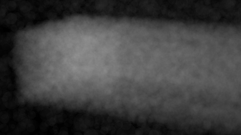
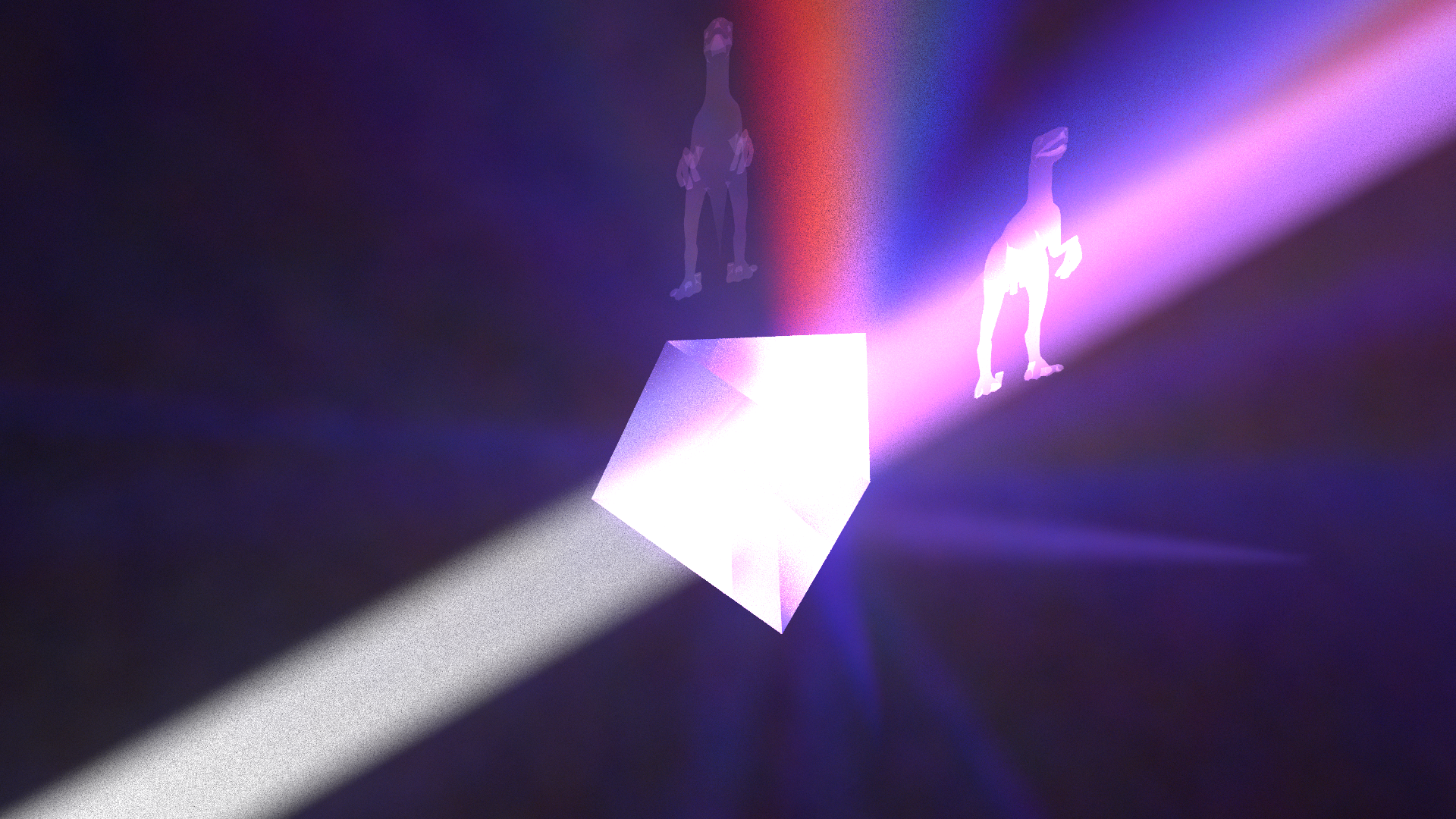
**Final project** (#) John “James” Utley (f004ghq) and Sam Morton (F0031W1) (##) Motivational image  This is our first motivational image. It demonstrates the type of fog objects that we want to color with the rainbow.  This is our second motivational image. It shows how we want to shine light through a prism to create a rainbow. We want to shine a light through a prism and have the different colors of the rainbow illuminate different objects which are made of fog. This conforms with the “Coloring Outside the Lines” theme because we are going to be coloring objects that don’t really have defined boundaries. (##) Volumetric Photon Mapping!  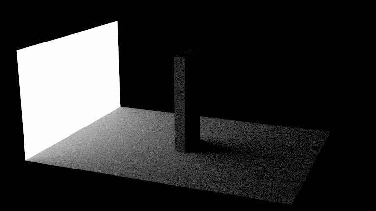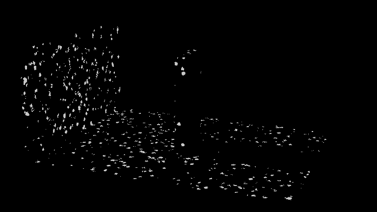This is the image of the scene we were first trying to render with just fog. Our first objective was to do some basic volumetric photon mapping with homogeneous media and global fog. With our end goal in mind we thought that we would not have to bother with surface photon mapping as nothing in our scene would be made of a material that could use surface photons. We had our light, a prism which was spectral, and various objects made of fog which would all use volumetric photon mapping. Starting with the Odyssey Scene, we quickly set up a first and second pass. The first pass was intended to distribute photons among the fog and the second was made in order to go out and detect those photons. We made outlines of both the first and second passes but we decided to start by implementing the first pass. Instead of emitting light from the emissive surfaces based on the typical cosine sampling where light from a surface could go in all sorts of directions we instead sampled a random position on emissive surfaces and then sent the photons in the direction of the surface normal. This had the intended effect of sending all our photons in the same direction, which would be important later in order to make the effect of different inidces of refraction for different wavelengths more pronounced. In order to simulate the particles in our homogeneous media we implemented a greenstein function which is a distribution function for how light scatters when it hits a scattering particle. We unfortunately do not sample from a greenstein function and instead sample from a random direction on a sphere. This has the effect of greatly reducing the power of photons when they bounce in a direction which is unlikely according to the greenstein function leading to some wasted photons. In the second pass we used ray marching to figure out the amount of radiance from any direction. We took fixed sized steps along the rays and used a fixed sized kernel in the shape of sphere to get the density of all the nearby photons. To speed up rendering times so that we could iterate faster we implemented a max ray length and a min ray length. We would then adjust these for each scene to minimize rendering times because we would end up marching no matter if we had any light in the area or not. This would work fairly well because our light was always concentrated into beams. However, when first implementing volumetric photon mapping we set the distances wrong and kept getting really weird renderings which took us too long to figure out.  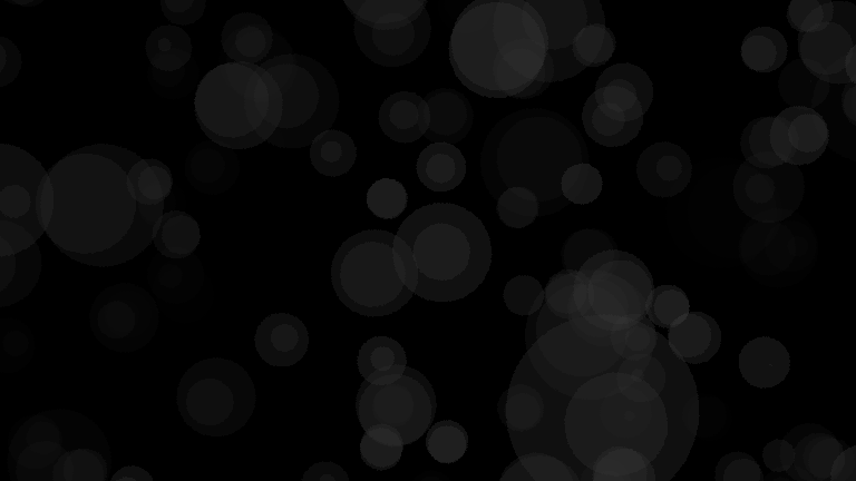This is what we kept getting stuck on. We eventually started implementing surface photon mapping, starting with a second pass that used volumetric photons and discvoered alot more photons were being placed than we were displaying, which finally lead us to figure out that had simply had max distance set too low.  Surface Photon mapping using out volumetric photons.  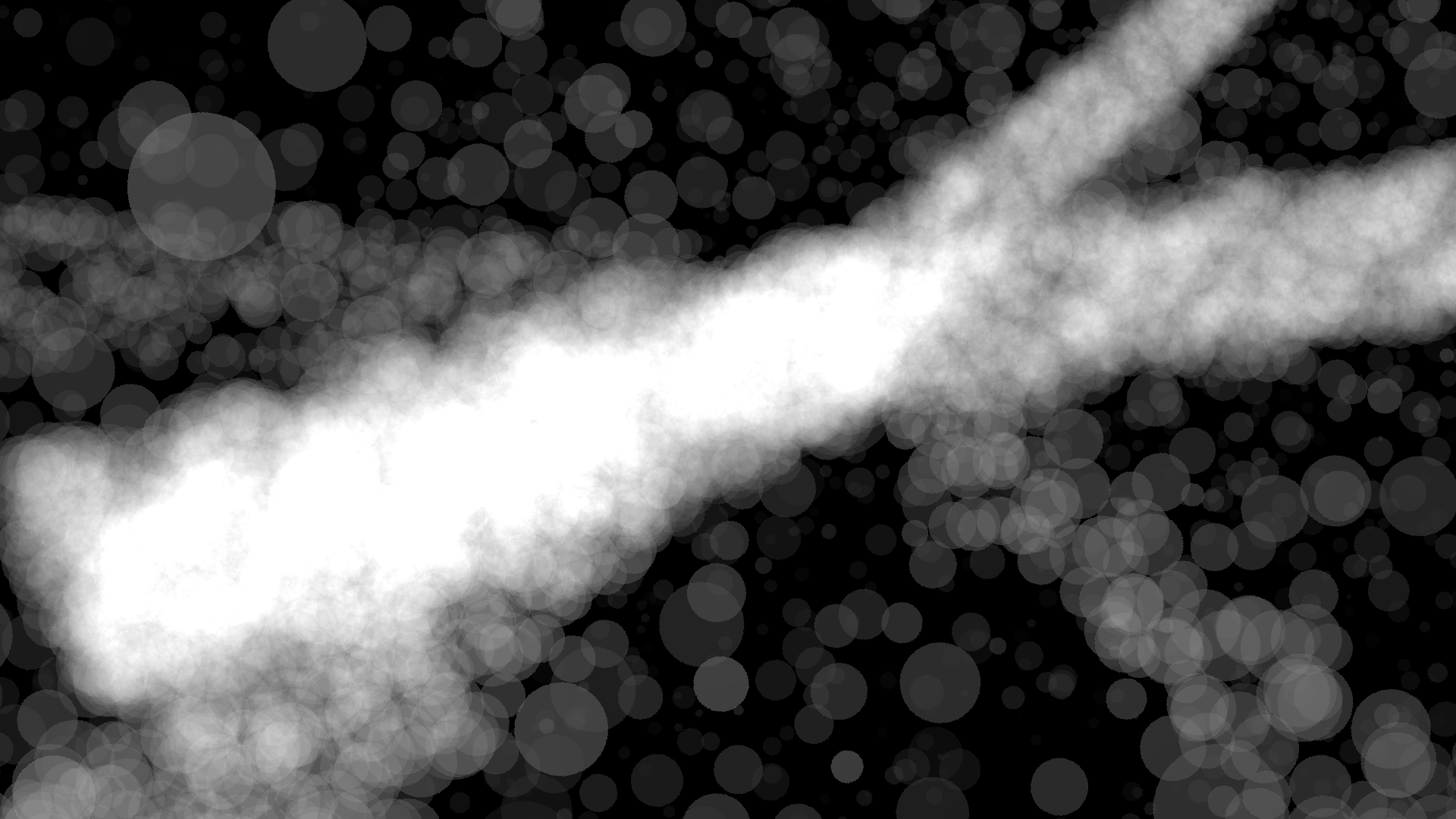This is what we finally got and our desired volumetric photon mapping. This rendering shows a working homogeneous global volumetric photon mapping. We can tell it is working by the few photons outside of the beam and the way that the beam is decaying as it travels through the fog. (##) Bounding To Shapes A brief note on bounding our volumetric photon mapping to shapes. For our implementation, we used the structure already laid out in lab 3 for generating custom shapes in our images, but there are important nuances we encountered which must be noted. First, given our focus on volumetric photon mapping with participating media, we wanted to implement our scenes containing a "default" medium which served as the basic medium which was visible throughout the image. This allowed us to control the transmittance and general appearance of the image environment, before we added additional surfaces or media. For example, this would allow us make the entire image "foggy" as opposed to completely clear, as would be the default. The next implementation note is that, in order to incorporate volumetric photon mapping and participating media with rendered meshes, we needed a way for materials to associate with a medium. Further, the material of the shapes we wanted to render in our final image was actually unimportant for the purpose of rendering, as the shapes were to be composed entirely of media. Thus, we decided to implement a new "generic material" (implemented in medium_material.cpp) which would essentially track the medium associated with the shape in question, and enable operations with that media. This way, the medium of a material could be taken into account when estimating radiance. Each medium we associated with a shape was a homogeneous medium, and thus we could define this in the json file. Thus, each shape mesh we defined in the json file could be associated with its own homogenous medium with custom parameters. In order to render realistic light interactions with our volumes, we needed to make a further extension to the ray marching algorithm we implemented. Specifically, we needed camera rays to be aware of when they penetrated the membrane of a new medium. For example, if the ray were traveling through air (also implemented as a default medium in our scene) and then entered fog, it would need to be aware of the new medium it was traveling through and the implications for its transmittance. We addressed this added complexity in the following manner: 1) the ray would march along until its first intersection. 2a) in the case that the ray has intersected with a wavelength material, we sample a new direction from the BSDF of the material with a wavelength of 550nm, which is the middle of the human-visible spectrum. 2b) In the case that the ray intersects with the "generic material", ray marching continues, but with a new ray starting at the intersection point and pointing in the same direction as the original ray.  (###) Russian Roulette We implemented Russian Roulette as a strategy for both increasing the efficiency of our code and for maintaining the power of the photons we were mapping. Our implementation is relatively straightforward and follows the Russian Roulette algorithm as it was described in lecture. It can be toggled on and off in our json files, but defaults to being on. Effectively, at each point in which we shoot photons, we first check if Russian Roulette is enabled. If it is enabled, then obtain the probability of shooting the photon (vs. returning early), and renew the photon's power if it is to be sent. (##) Prism Refraction and Making a Rainbow! To set up some faux spectral rendering we first needed a good test scene. So we took a prism and put it front of a square light source. The idea was to create angles so that different indices of refraction would result in drastically different angles for the different color photons.  This is our test scene that we wanted to use to eventually make a rainbow. First order of business was to make the photons refract at all. That was pretty straightforward we just sampled from our already completed dialectric materials when we hit them.  Here is the first working refraction for photons (##) Modeling Human Vision Receptors We then had to seperate the photons by wavelength. The two major hurdles for our faux spectral rendering were first converting wavelengths into colors and second using wavelengths to determine new indices of refraction. The first problem was solved when we found a very helpful blog post that broke down how humans perceive different wavelengths and how that could be used for spectral rendering. Humans have 3 visual recepetors, conveniently a receptor for Red, Green, and Blue, these receptors have varying sensitivities over the visible wavelength spectrum which gives us all of the colors we know and love and results in the classic rainbow (Zhang). We can use 3 normal distributions in order to model the receptor's sensitivity to light at various wavelengths (Zhang). In the blog post those 3 normal distributions were given via a distribution mean and a standard deviation, we ended up using those distributions.  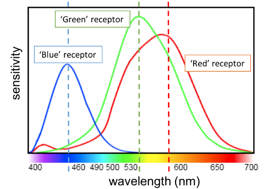Here's an image from the blog post showing the receptors and their sensitivity to light at different wavelengths. In order to model those distributions we grabbed the formula to evaluate the gaussian at any point from wikipedia.  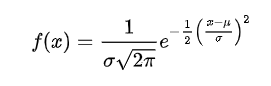Formula from wikipedia. Then in order to evaluate the color of a wavelength, we evaluated the 3 gaussian distributions and scaled the red green and blue channels of a pure white by the value of the gaussian distribution for that channel's receptor at that wavelength. We then took the remaining color and normalized it so no matter what wavelength you took it would have the same luminance. This was a dicey thing to do as there are clearly darker areas on the traditional rainbow but it stopped the wavelength sections where the gaussians were all low from becoming very dark, so we believe it was a trade worth making as most of the rainbow is very light. We also added a fourth distribution in order to model the small amount of red at the low end of the visible light spectrum which gives rise to purple. To get this distribution we just eye balled it, using both guess and check as well as the small bump in the graph from the blog as a guide. This ended up as pink because we normalize the luminance, so it would be impossible to get a true purple using our system. Pink is better than nothing though. Another issue with our approximation of human vision is that the receptors all have different max sensitivities but we had them all be the same height this obviously lead to some bias.  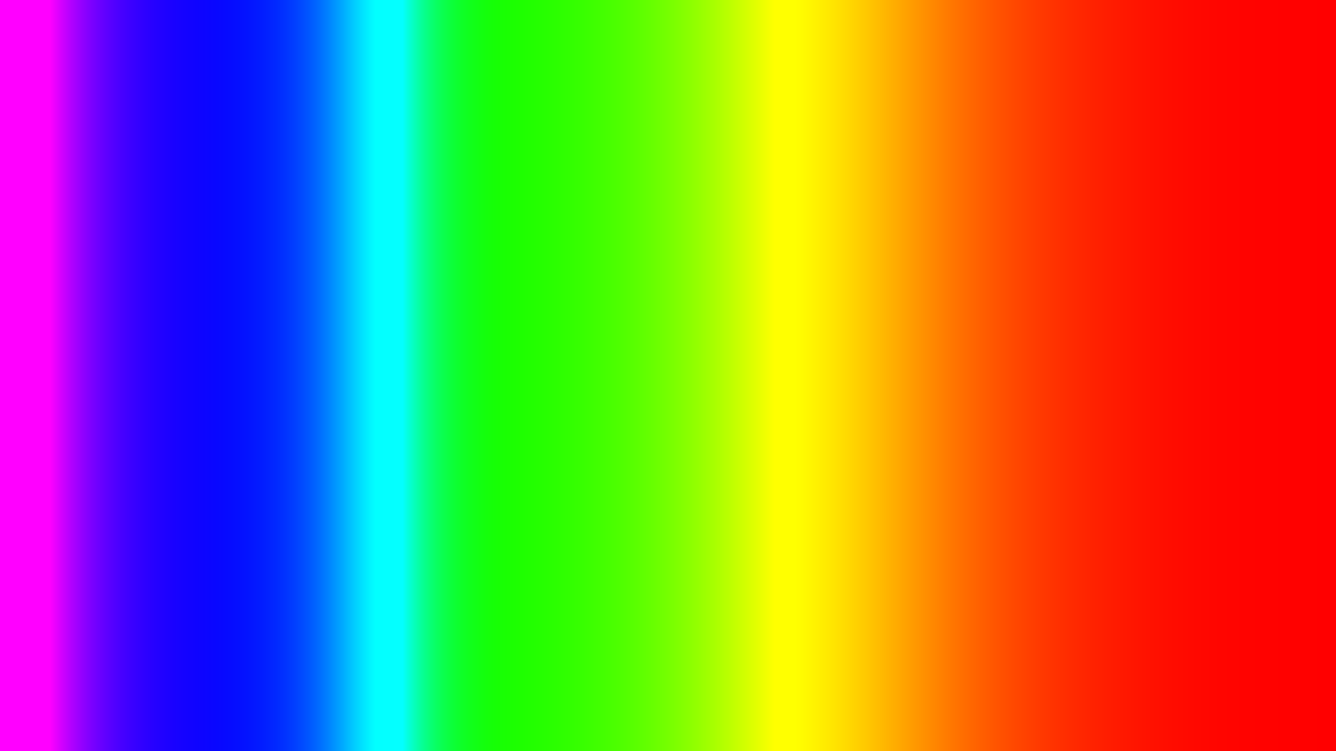This is the end result of our conversion from wavelength to color. Our approximation of the rainbow was clearly not perfect. Doing a sanity check revealed that the rainbow was biased towards a pinkish color when it should have been a perfect white with all the wavelengths combined. We emitted our photons with no wavelength attached to them and then assigned them a wavelength when it was absolutely needed, likely for refraction. Once a photon was assigned a wavelength that wavelength would remain with the photon until it finished all of its bounces. This made it so that a photon with a particular wavelength would always bounce using the same index of refraction as it would in real life. When light was deposited into our volumetric tree, we simply took the light that the photon was and multiplied it by the wavelength color it should be, this was fine as it retained it's original luminance because our rainbow is normalized.  Changing color when we split the wavelengths (##) Changing Index of Refraction based on Wavelength We then moved onto the second hurdle where we had to convert wavelengths into various indices of refraction for materials. We found lots of methods for doing this online. In the blog referenced earlier they just had a function that found statistically and they just looked up into that function. This was obviously not an option for us. Instead we found a short study guide for high school level physics which gave us a great approximation of wavelength varying indexes of refractions which obviously wasn't perfect because real life materials are much more complicated. The formula was W1 * N1 = W2 * N2 (study.com). Where W's are wavelengths and N's are indices of refraction. So using this as long as we knew one index of refraction for one wavelength we could calculate the index of refraction to a fair approximation at any other wavelength. We decided to just use the wavelength at 550 nanometers to specify our index of refraction at. Then using that as a baseline we calculated all other indices of refraction when they were needed for various photons.  Here is the light splitting based on the index of refraction! (##) Randomized Marching In the previous picture you can see some artifacts due to our ray-marching algorithm. This is because we always take the same sized steps with each march, meaning we are gonna jump over the beam in the same way for every pixel. To avoid this we originally randomized our march step sizes slightly but we found this still produced some artifacts just less noticable. In order to truly get rid of all the artifacts we take equal steps but sample from the fog from random places in those steps. This produces a much cleaner image.  Cleaner prism with random marching. (##) Attempt at Heterogenous Media The initial idea of the project was to compose the objects of homogeneous fog and then have a more whimsical for globally. We thought this might correspond to perlin noise. Alas, we kept getting very regular patterns when we tried to use the noise functions given to us. It did give us some cool renderings though even if we ended up scrapping heterogeneous media.  (##) Surface Photon Mapping! After completing the faux spectral rendering and the volumetric rendering we wanted to add some extra functionality and landed on completing our surface photon mapping. If you remember we partially implemented the second pass of this in order to test the volume so all we had to do was add a first pass and finish the second pass. The first pass was more complicated than it needed to be. We ended up redoing lambertian sampling and ortho normal basis to get it working. Whenever we hit a lambertian surface instead of killing off the photon immediately we instead bounce the photon off of the surface according to the BRDF and leave a photon deposit on the surface. This deposit is made in a seperate tree from the volumetric deposits so that we can distinguish the two types. The second pass then does normal marching to get the radiance due to in scattering along a ray but at the end of it's marching it checks the surface that it hits and uses the surface deposits to estimate the light on the surface. After finding the light traveling along the ray directly from the surface it modifies it by the transmittance between the surface and the camera. This results in surface photon mapping through homogeneous medium. It is important to note that the surface photons are only applying to lambertian surfaces in our scenes. Spectral surfaces like the prism will not have photons deposited on them and really only serve to redirect the photons.  Here is our first working photon mapping scene (##) Surface Mapping With Colors The next thing to do was to make sure that albedo was working for surface photons. So everytime we bounced we multiplied the power of the photon bouncing by the albedo of the object that it was bouncing off of. We also took the final deposit and multiplied it by the albedo of the object it landed on, this is because it was effectively making a bounce to travel along the camera ray.  This is a rendering demonstrating photons being modified by the albedos of the walls which they hit. Finally, we added back our global fog to our scene here and it worked suprisingly well. You'll notice that our surface photon mapping suffers from similar issues that most surface photon mapping suffers from. Mainly splotchiness and bias. Bias can be seen in the edges of the room where it gets much darker and bias can be seen in the direct lighting where a square light is blurred to have rounded corners.  Surface photon mapping and volumetric photon mapping in one scene! (##) Spectral Surface Colors Limitation Adding the surface mapping did come with some issues though. It made our faux spectral work obsolete. This is because we handle albedo by simply multiplying by the power of photons by the albedo of objects we bounce off of, no matter what wavelelength our photon is. This means that a pink photon can bounce off a green wall and deposit a green-pink some where else in the scene. This should not be possible, a pink photon should always remain pink but that is unfortunately not the case. (##) Spectral Camera Ray Limitation Another limitiation is that we did not extend the camera rays to have spectral refraction. No matter what camera rays will bounce through wavelength materials as if they were a photon with a wavelength of 550 nanometers. This is bad because it means that as soon as light has been gathered from deposits and is traveling back to the camera ray it losses it's property of different indices of refraction for different wavelengths. (##) Final Rendering Our final image was generated via extensive tinkering between Blender and the outputted json file. We will admit that we had a lot of trouble properly exporting our scenes, as well as properly orienting our prism to get the best rainbow. We would now like to present... our final image!  (##) Bibliography “Spectral Ray Tracing.” CECILIA ZHANG, https://ceciliavision.github.io/graphics/a6/#part2. “Normal Distribution.” Wikipedia, Wikimedia Foundation, 16 Nov. 2022, https://en.wikipedia.org/wiki/Normal_distribution. “Take Online Courses. Earn College Credit. Research Schools, Degrees & Careers.” Study.com | Take Online Courses. Earn College Credit. Research Schools, Degrees & Careers, https://study.com/skill/learn/how-to-calculate-the-index-of-refraction-of-a-medium-using-wavelength-change-explanation.html.