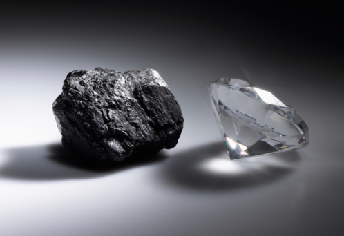
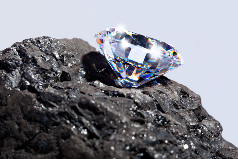
Inspiration Images
Diamonds are made from carbon, but the appearance of these two items are totally different. So I think the diamond and carbon go well to the theme "Contrast". And I started off with the following inspiration images shown below, a diamond on a big carbon bed or a contrast scene between the diamond and carbon.
Inspiration Image
Features
SpotLight
Spotlight is a pointlight which only shines in a certain direction. The consept of a spot light can be thought of light ol shining through a cone. I made the borders of the cone are not sharp, there is a certain boundary in which the light intensity fades. One parameter determines the cosine of the begining of the fade(F) angle of the cone, where the full intensity of the emitter is received. The other parameter determines the cosine of the angle of the total width(W) of the cone. At any angles larger than this, the received radiance from this light source is zero.In between the two angles, the intensity linearly decreases, which gives the smooth border effect. The function fade() computes the transition range from the center of the cone to the outside, which is totaly black. This implementation works for photon mapping as well. In order to sample a direction from the spotight, I used the function Warp::squreToUniformSphereCap(). Implementation mainly forcused on spotLight.cpp file
Spotlight parameters:
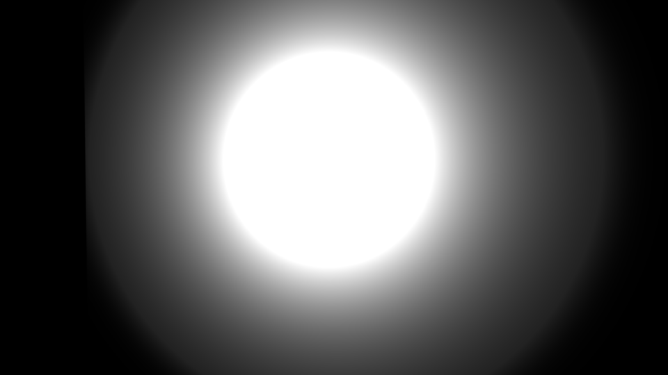
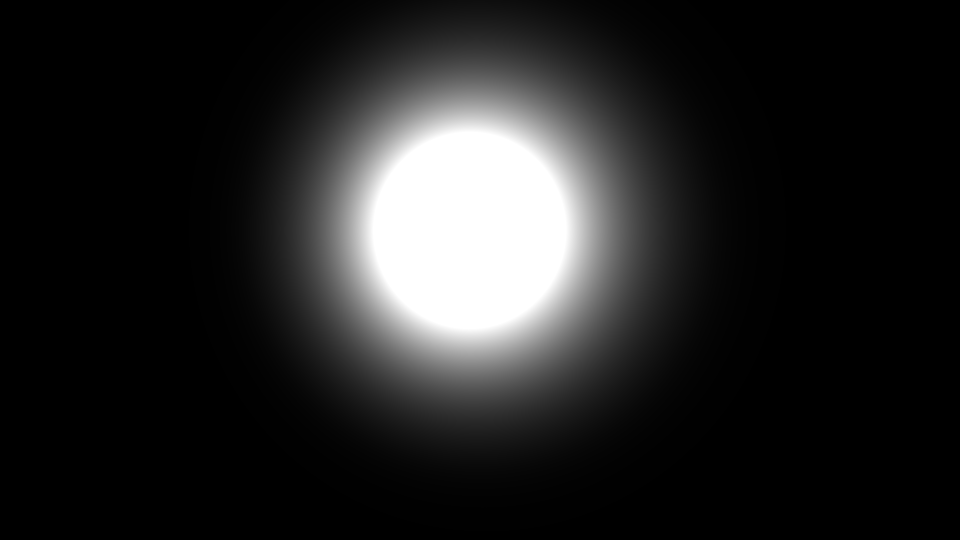
Below we can see four example images for the spot light. In the first two, we can see the comparison of a spot light with soft border and hard borders. In the latter case, F = W, which means that there is no room for a smooth transition.
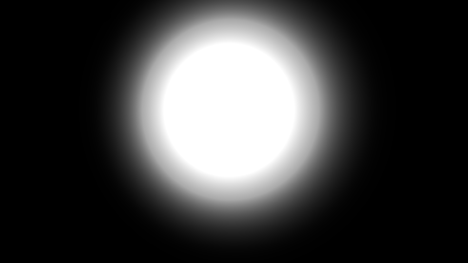
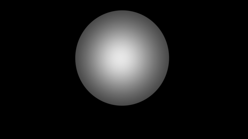
In these two images, the total width (W) of the cone is very large. Here, we can se a comparison between a large falloff angle (cosine = .4) and a smaller falloff angle (.95).
Depth of Field
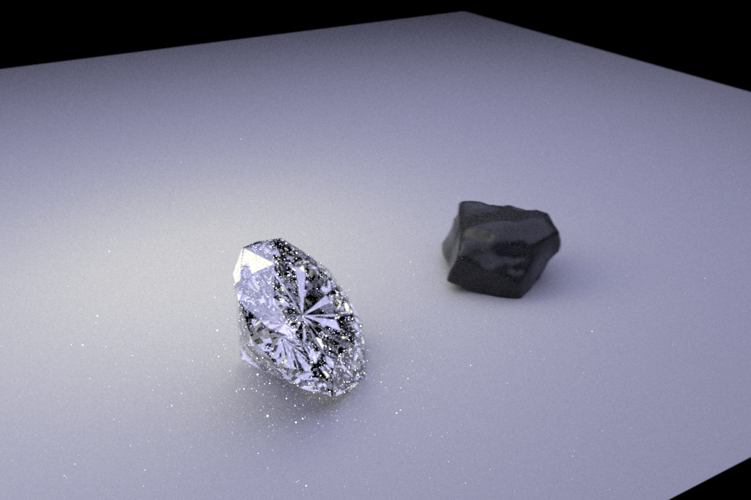
The Dof feature determines the range of distances within which objects appear in focus. Implementation:Implemented this feature based on the perspective camera code. Integration over pixel area and aperture area. Typically, the lens geometry is defined by the radius and the distance to the focal plane.Sample the aperture, figure out the outgoing direction so that the points on the focal plane are in focus.The following two pictures show the scene with/without Dof feature.Implementation mainly forcused on DoFCamera.cpp file.(I got the 3D obj files from http://www.turbosquid.com/Search/3D-Models/free/obj)

Progressive Pohton Mapping
From the convergence analysis, we know that the Noise of average will descrease with the kernal size shrinked and also the Bias of average will decrease.So progressively shrink the density estimation kernel could reduce the noise of the rendered picture. Implementation: Parameter Set:alpha = 2/3; Step1: Photon tracing: emit,scatter,store photons; Step2: Trace camera paths and evaluate radiance estimate using ri; After these two steps, display runing average. Using this formula to compute new radius:
$$ r^2_{i+1} = \frac{i+\alpha}{i+1}r^2_i $$The following pictures are selected rendered images with shrinking radius, which we can see that the radius are shrinking. To see the performance of progressive photon mapping more apparently and make the rendering process more faster(100 images need to render), I set the number of photons to be 50000.Implementation mainly forcused on two part: photonmapper.cpp and average folder(image average code).
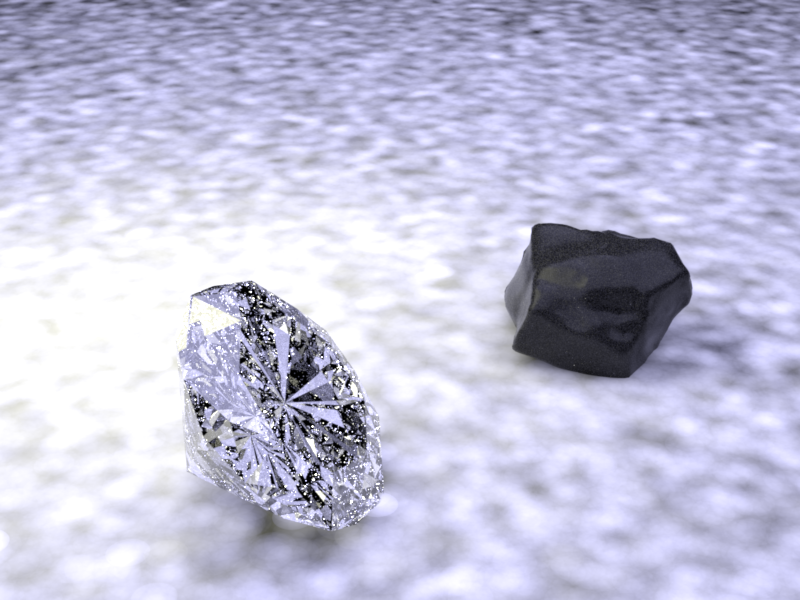

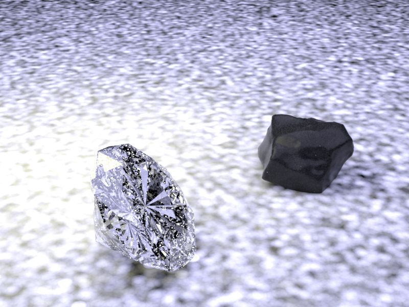


The following two pictures show the comparison between the original image and the averaged images. We can see that it's clear the carbon appearance is better than the original image.


Dispersion Rendering
The brilliance,fire,gleaming are the main reason of diamond's brilliance, so I generated the dispersion redering feature to make the rendered diamond more realism. Real light is composed of a spectrum of wavelengths,to reproduce the color fringing on the diamond,there are two broad approaches to spectral rendering: binning, and Monte Carlo spectral sampling. Both approaches have their pros and cons.Finally, I chosed the latter method to do the dispersion Rendering.The Monte Carlo approach has one big down side: color noise. Below is a spectral render of a solid medium-gray background with one sample per pixel, 16 samples per pixel.
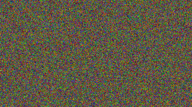

In the Monte Carlo approach, colors don't have a single canonical way to be represented. However, that is also one of the pros of the Monte Carlo approach: you can have many different ways to represent color, and as long as they can all be sampled spectrally, they can all coexist effortlessly within the same renderer. Monte Carlo sampling is also more accurate than binning. For example, if you rendered a scene with a prism, the resulting image from a binning approach would only have as many colors as there are bins. But a Monte Carlo approach would, when converged, reveal all the colors of the rainbow in a smooth gradient. Finally, the Monte Carlo approach takes up less memory (only one value instead of 9-30), and might be faster depending on a variety of factors.
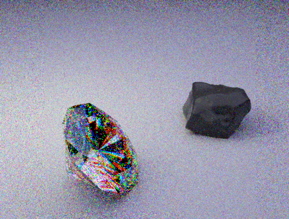
Algorithm: with each sample path , generate 3 paths with RGB wavelength separately and then trace those paths, finally add them together to get the rendered result. In this process, each wavelength will have different IOR. Implementation: Mainly focused on these two files: linear_spectral_dielectric.cpp and RGB.cpp
The following two images show the noise color apparance in the begining and the dispersion rendered result image.
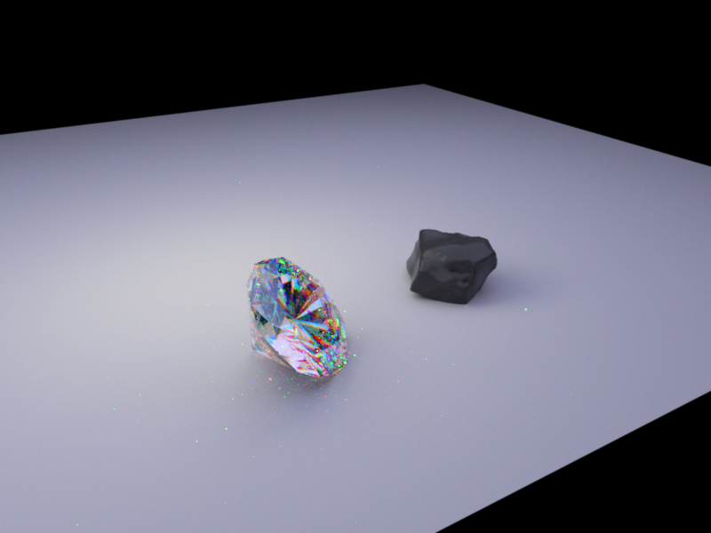
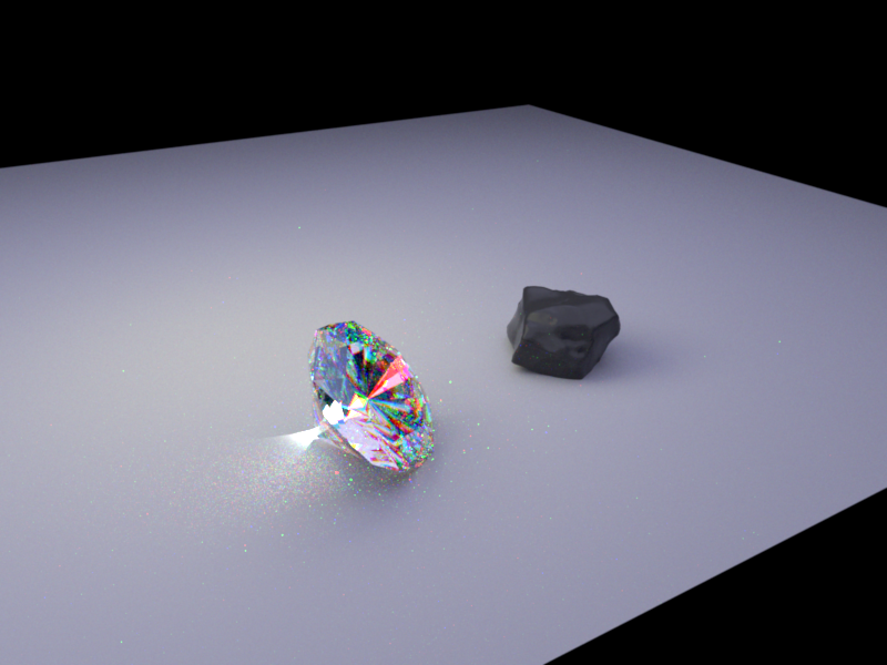
Final Rendered Image
Originally, I want to render this scene mainly based on photon mapping, so I generated the feature progressive photon mapping, and I also want to add another advaced feature: use parametric way of estimating the probability density of a random variable (photon density). But I finally failed. So I chose to use the dispersion rendering result added the spot light scene as the final result picture shown below.
