You have probably seen big-Oh notation before, but it's certainly worthwhile to recap it. In addition, we'll see a couple of other related asymptotic notations. Chapter 4 of the textbook covers this material as well. I strongly suggest reading it.
Remember back to linear search and binary search. Both are algorithms to search for a value in an array with n elements. Linear search marches through the array, from index 0 through the highest index, until either the value is found in the array or we run off the end of the array. Binary search, which requires the array to be sorted, repeatedly discards half of the remaining array from consideration, considering subarrays of size n, n/2, n/4, n/8, …, 1, 0 until either the value is found in the array or the size of the remaining subarray under consideration is 0.
The worst case for linear search arises when the value being searched for is not present in the array. The algorithm examines all n positions in the array. If each test takes a constant amount of time—that is, the time per test is a constant, independent of n—then linear search takes time c1n + c2, for some constants c1 and c2. The additive term c2 reflects the work done before and after the main loop of linear search. Binary search, on the other hand, takes c3 log2 n + c4 time in the worst case, for some constants c3 and c4. (Recall that when we repeatedly halve the size of the remaining array, after at most log2 n + 1 halvings, we've gotten the size down to 1.) Base-2 logarithms arise so frequently in computer science that we have a notation for them: lg n = log2 n.
Where linear search has a linear term, binary search has a logarithmic term. Recall that lg n grows much more slowly than n; for example, when n = 1,000,000,000 (a billion), lg n is approximately 30.
If we consider only the leading terms and ignore the coefficients for running times, we can say that in the worst case, linear search's running time "grows like" n and binary search's running time "grows like" lg n. This notion of "grows like" is the essence of the running time. Computer scientists use it so frequently that we have a special notation for it: "big-Oh" notation, which we write as "O-notation."
For example, the running time of linear search is always at most some linear function of the input size n. Ignoring the coefficients and low-order terms, we write that the running time of linear search is O(n). You can read the O-notation as "order." In other words, O(n) is read as "order n." You'll also hear it spoken as "big-Oh of n" or even just "Oh of n."
Similarly, the running time of binary search is always at most some logarithmic function of the input size n. Again ignoring the coefficients and low-order terms, we write that the running time of binary search is O(lg n), which we would say as "order log n," "big-Oh of log n," or "Oh of log n."
In fact, within our O-notation, if the base of a logarithm is a constant (such as 2), then it doesn't really matter. That's because of the formula
loga n = logb n / logb a
for all positive real numbers a, b, and c. In other words, if we compare loga n and logb n, they differ by a factor of logb a, and this factor is a constant if a and b are constants. Therefore, even when we use the "lg" notation within O-notation, it's irrelevant that we're really using base-2 logarithms.
O-notation is used for what we call "asymptotic upper bounds." By "asymptotic" we mean "as the argument (n) gets large." By "upper bound" we mean that O-notation gives us a bound from above on how high the rate of growth is.
Here's the technical definition of O-notation, which will underscore both the "asymptotic" and "upper-bound" notions:
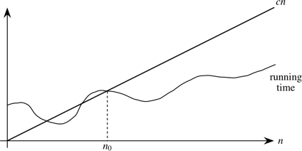
A running time is O(n) if there exist positive constants n0 and c such that for all problem sizes n ≥ n0, the running time for a problem of size n is at most cn.
Here's a helpful picture:
The "asymptotic" part comes from our requirement that we care only about what happens at or to the right of n0, i.e., when n is large. The "upper bound" part comes from the running time being at most cn. The running time can be less than cn, and it can even be a lot less. What we require is that there exists some constant c such that for sufficiently large n, the running time is bounded from above by cn.
For an arbitrary function f(n), which is not necessarily linear, we extend our technical definition:
A running time is O(f(n)) if there exist positive constants n0 and c such that for all problem sizes n ≥ n0, the running time for a problem of size n is at most c f(n).
A picture:
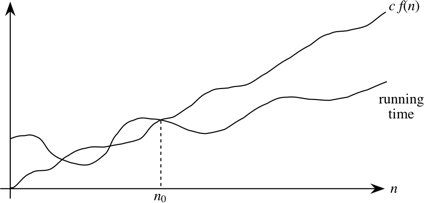
Now we require that there exist some constant c such that for sufficiently large n, the running time is bounded from above by c f(n)
Actually, O-notation applies to functions, not just to running times. But since our running times will be expressed as functions of the input size n, we can express running times using O-notation.
In general, we want as slow a rate of growth as possible, since if the running time grows slowly, that means that the algorithm is relatively fast for larger problem sizes.
We usually focus on the worst case running time, for several reasons:
You might think that it would make sense to focus on the "average case" rather than the worst case, which is exceptional. And sometimes we do focus on the average case. But often it makes little sense. First, you have to determine just what is the average case for the problem at hand. Suppose we're searching. In some situations, you find what you're looking for early. For example, a video database will put the titles most often viewed where a search will find them quickly. In some situations, you find what you're looking for on average halfway through all the data…for example, a linear search with all search values equally likely. In some situations, you usually don't find what you're looking for.
It is also often true that the average case is about as bad as the worst case. Because the worst case is usually easier to identify than the average case, we focus on the worst case.
Computer scientists use notations analogous to O-notation for "asymptotic lower bounds" (i.e., the running time grows at least this fast) and "asymptotically tight bounds" (i.e., the running time is within a constant factor of some function). We use Ω-notation (that's the Greek leter "omega") to say that the function grows "at least this fast". It is almost the same as Big-Oh notation, except that is has an "at least" instead of an "at most":
A running time is Ω(f(n)) if there exist positive constants n0 and c such that for all problem sizes n ≥ n0, the running time for a problem of size n is at least c f(n).
We use Θ-notation (that's the Greek letter "theta") for asymptotically tight bounds:
A running time is Θ(f(n)) if there exist positive constants n0, c1, and c2 such that for all problem sizes n ≥ n0, the running time for a problem of size n is at least c1 f(n) and at most c2 f(n).
Pictorially,
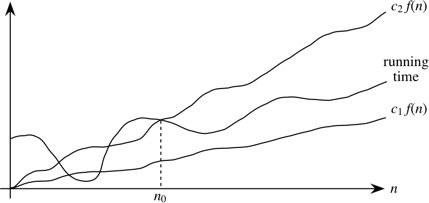
In other words, with Θ-notation, for sufficiently large problem sizes, we have nailed the running time to within a constant factor. As with O-notation, we can ignore low-order terms and constant coefficients in Θ-notation.
Note that Θ-notation subsumes O-notation in that
If a running time is Θ(f(n)), then it is also O(f(n)).
The converse (O(f(n)) implies Θ(f(n))) does not necessarily hold.
The general term that we use for O-notation, Θ-notation, and Ω-notation is asymptotic notation.
Asymptotic notations provide ways to characterize the rate of growth of a function f(n). For our purposes, the function f(n) describes the running time of an algorithm, but it really could be any old function. Asymptotic notation describes what happens as n gets large; we don't care about small values of n. We use O-notation to bound the rate of growth from above to within a constant factor, and we use Θ-notation to bound the rate of growth to within constant factors from both above and below. (We won't use Ω-notation much in this course.)
We need to understand when we can apply each asymptotic notation. For example, in the worst case, linear search runs in time proportional to the input size n; we can say that linear search's worst-case running time is Θ(n). It would also be correct, but slightly less precise, to say that linear search's worst-case running time is O(n). Because in the best case, linear search finds what it's looking for in the first array position it checks, we cannot say that linear search's running time is Θ(n) in all cases. But we can say that linear search's running time is O(n) in all cases, since it never takes longer than some constant times the input size n.
Although the definitions of O-notation an Θ-notation may seem a bit daunting, these notations actually make our lives easier in practice. There are two ways in which they simplify our lives.
I won't go through the math that follows in class. You may read it, in the context of the formal definitions of O-notation and Θ-notation, if you wish. For now, the main thing is to get comfortable with the ways that asymptotic notation makes working with a function's rate of growth easier.
Constant multiplicative factors are "absorbed" by the multiplicative constants in O-notation (c) and Θ-notation (c1 and c2). For example, the function 1000 n2 is Θ(n2) since we can choose both c1 and c2 to be 1000.
Although we may care about constant multiplicative factors in practice, we focus on the rate of growth when we analyze algorithms, and the constant factors don't matter. Asymptotic notation is a great way to suppress constant factors.
When we add or subtract low-order terms, they disappear when using asymptotic notation. For example, consider the function n2 + 1000 n. I claim that this function is Θ(n2). Clearly, if I choose c1 = 1, then I have n2 + 1000 n ≥ c1 n2, and so this side of the inequality is taken care of.
The other side is a bit tougher. I need to find a constant c2 such that for sufficiently large n, I'll get that n2 + 1000 n ≤ c2 n2. Subtracting n2 from both sides gives 1000 n ≤ c2 n2 − n2 = (c2 − 1) n2. Dividing both sides by (c2 − 1) n gives $\displaystyle \frac{1000}{c_2 - 1} \leq n$. Now I have some flexibility, which I'll use as follows. I pick c2 = 2, so that the inequality becomes $\displaystyle \frac{1000}{2-1} \leq n$, or 1000 ≤ n. Now I'm in good shape, because I have shown that if I choose n0 = 1000 and c2 = 2, then for all n ≥ n0, I have 1000 ≤ n, which we saw is equivalent to n2 + 1000 n ≤ c2 n2.
The point of this example is to show that adding or subtracting low-order terms just changes the n0 that we use. In our practical use of asymptotic notation, we can just drop low-order terms.
In combination, constant factors and low-order terms don't matter. If we see a function like 1000 n2 − 200 n, we can ignore the low-order term 200 n and the constant factor 1000, and therefore we can say that 1000 n2 − 200 n is Θ(n2).
As we have seen, we use O-notation for asymptotic upper bounds and Θ-notation for asymptotically tight bounds. Θ-notation is more precise than O-notation. Therefore, we prefer to use Θ-notation whenever it's appropriate to do so.
We shall see times, however, in which we cannot say that a running time is tight to within a constant factor both above and below. Sometimes, we can bound a running time only from above. In other words, we might only be able to say that the running time is no worse than a certain function of n, but it might be better. In such cases, we'll have to use O-notation, which is perfect for such situations.
Big Θ-notation can help predict running times for big data sets based on the run times for small data sets. Suppose you have a program that runs the insertion sort algorithm, whose worst and average case run times are Θ(n2), where n is the number of items to sort. Someone has given you a list of 10,000 randomly ordered things to sort. Your program takes 0.1 seconds. Then you are given a list of 1,000,000 randomly ordered things to sort. How long do you expect your program to take? Should you wait? Get coffee? Go to dinner? Go to bed? How can you decide?
The expected run time for insertion sort on random data is Θ(n2). The means that the run time approaches cn2 asymptotically, or is at least upper-bounded by such an expression. 10,000 is fairly big - the lower-order terms shouldn't have much effect. Therefore we approximate the actual function for the run time by f(n) = cn2.
There are two ways we can solve this. The more straighforward way (and the way that will work for run times like Θ(n log n)) is to solve for c:
f(10,000) = c 10,0002 = 0.1
c = 0.1/(104)2 = 10-9
Therefore we can approximate f(n) as:
f(n) = 10-9n2
Plugging in n = 1,000,000 we get:
f(1,000,000) = 10-9 (106)2 = 1000
We therefore estimate 1000 seconds or a 16.666 minutes. Time enough to get a cup of coffee, but not to go to dinner.
We can use a shortcut for polynomials. If the run time is approximately cnk for some k, then what happens to the run time if we change the input size by a factor of p? That is, the old input size is n and the new input size is pn. Thus if
f(n) = cnk
thenf(pn) = c(pn)k = pkcnk = pkf(n)
Therefore changing the input size by a factor of p changes the run time by a factor of pk. In the problem I gave you, p = 1,000,000/10,000 = 100 and k = 2, so the run time changes by a factor of 10,000. So the time is 10,000 times 0.1, or 1000 seconds.
Suppose that you were running mergesort instead of insertion sort in the example above. Merge sort's run time is Θ(n log n). We approximate the run time as f(n) = cn log n. Note that log210,000 = 13.29. Solving for c gives:
f(10,000) = c 10,000 log 10,000 = c 10,000 (13.29) = 0.1
c = 0.1/132,900 = 7.52 x 10⁻⁷
f(n) = (7.53 x 10⁻⁷) n log n
Plugging in n = 1,000,000 and using the fact that log 1,000,000 is a bit less than 20 gives:
f(1,000,000) = (7.53 x 10⁻⁷) 1,000,000 log 1,000,000 = .753 x 20 = 15.05 So the run time in this case is 15 seconds. Might as well wait for it to finish.A stack is a LIFO (Last In, First Out) data structure. The book compares a stack to a spring-loaded stack of cafeteria trays or a PEZ dispenser. (Though I have to question how well the authors remember PEZ. They are candies, but definitely not mint.) The abstract data type (ADT) Stack has at least the following operations (in addition to a constructor to create an empty stack):
push: add to the top of the stackpop: remove the top element from the stack and return itpeek: return the top element but do not remove itisEmpty: return a boolean indicating whether the stack is emptySo what good is a stack? It has many, many applications. You already know that the run-time stack handles allocating memory in method calls and freeing memory on returns. (It also allows recursion). A stack provides an easy way to reverse a list or string: push each element on the stack then pop them all off. They come off in the opposite order that they went on. They are good for matching parentheses or braces or square brackets or open and close tags in HTML.
A stack is also how HP calculators handle reverse Polish notation. In this notation the operator follows both operands, and no parentheses are needed. So the expression (3 + 5) * (4 - 6) becomes 3 5 + 4 6 - *. To evaluate it, push operands onto the stack when you encounter them. When you reach an operator, pop the top two values from the stack and apply the operator to them. (The first popped becomes the second operand in the operation.) Push the result of the operation back on the stack. At the end there is a single value on the stack, and that is the value of the expression.
A stack is also how you can do depth-first search of a maze or a graph. Let's consider a maze. Start by pushing the start square onto the stack. The repeatedly do the following:
Quit when you reach the goal square.
Because Stack is an ADT, an interface should specify its operations. The CS10Stack interface in CS10Stack.java contains the operations given above.
The class java.util.Stack also has these operations, but instead of the name isEmpty they use empty. It also has an additional operation, size.
The book has its own version of the ADT, but instead of the name peek they use top, and they also add size. You would think that computer scientists could agree on a standard set of names. Yeah, not so much. At least we all agree on push and pop.
One question is how to handle pop or peek on an empty stack. Both Java and the book throw an exception. That seems a bit harsh, and so CS10Stack is more forgiving: it returns null.
How do we implement a stack? One simple option is to use an array. The implementation has two instance variables: an array called stack and an int called top that keeps track of the position of the top of the stack. In an empty stack top equals − 1. To push, add 1 to top and save the value pushed in stack[top]. To peek just return stack[top] (after checking that top is nonnegative). pop is peek but with top--.
This implementation is fast (all operations take O(1) time), and it is space efficient (except for the unused part of the array). The drawback is that the array can fill up, and when it does, you get an exception on push.
An alternative that avoids that problem uses a linked list. A singly linked list suffices. The top of the stack is the head of the list. The push operation adds to the front of the list, and the pop removes from the front of the list. All operations are take O(1) time in this implementation, also. You need to have space for the links in the linked list, but you never have empty space as you do in the array implementation.
Another way that avoids the problem of the array being full is to use an ArrayList. To push, you add to the end of the ArrayList, and to pop you remove the last element. The ArrayList can grow, so it never becomes full. The code for this implementation is in ArrayListStack.java. Note that you don't even need to keep track of the top. The ArrayList does it for you.
Do these operations all take O(1) time? It looks like it, as long as add and remove at the end of the ArrayList take O(1) time. The remove operation certainly takes O(1) time. The add usually does is, but sometimes can take longer.
To understand why an add operation can take more than constant time, we need to look at how an ArrayList is implemented. The underlying data structure is an array. There is also a variable to keep track of the size, from which we can easily get the last occupied position in the array. Adding to the end just increases the size by 1 and assigns the object added to the next position. However, what happens when the array is full? A new array is allocated and everything is copied to the new array. Doing so takes time Θ(n), where n is the number of elements in the ArrayList.
If we had to copy the entire ArrayList upon each add operation, the process would be very slow. It would in fact take time O(n2) to add n elements to the end of the ArrayList. That would be too slow. So instead, when the ArrayList is full, the new array allocated is not just one position bigger than the old one, but much bigger. One option is to double the size of the array. Then a lot of add operations can happen before the array needs to be copied again.
With this approach, n add operations will take O(n) time. In other words, the average time per operation is only O(1). We call this the amortized time. Amortization is what accountants do when saving up to buy an expensive item like a computer. Suppose that you want to buy a computer every 3 years and it costs 1500 dollars. One way to think about this is to have no cost the first two years and 1500 dollars the third year. An alternative is to set aside 500 dollars each year. In the third year you can take the accumulated 1500 dollars and spend it on the computer. So the computer costs 500 dollars a year, amortized. (In tax law it goes the other direction: you spend the 1500 dollars, but instead of being able to deduct the whole thing the first year you have to spead it over the 3 year life of the computer, and you deduct 500 dollars a year.)
For the ArrayList case, we can think in terms of tokens that can pay for copying something into the array. Suppose that we have just doubled the array size from n to 2n, which means that we have just copied n elements; let's call these n elements that were copied the "old elements." We spend all our tokens copying the old elements, so that immediately after copying, we have no tokens available. By the time the array has 2n elements and the array size doubles again, we must have one token for each of the 2n elements to pay for copying 2n elements.
Here's how we do it. We charge three tokens for each add:
Therefore, by the time the array has 2n elements, every element has a token, which pays for copying it.
By thinking about it in this way, we see that the cost per add operation is a constant (three tokens).
The array size does not have to double when the array fills. For example, it could increase by a factor of 3/2, in which case you can modify the argument to show that charging four tokens per add operation works.
A Queue is a FIFO (First In, First Out) data structure. "Queueing up" is a mostly British way of saying standing in line. And a Queue data structure mimics a line at a grocery store or bank where people join at the back, are served when they get to the front, and nobody is allowed to cut into the line. The ADT Queue has at at least the following operations (in addition to a constructor to create an empty Queue):
enqueue: add an element at the rear of the queuedequeue: remove and return the first element in the queuefront: return the first element but don't remove itisEmpty: return a boolean indicating whether the queue is emptyWhat do we use a Queue for? An obvious answer is that it is useful in simulations of lines at banks, toll booths, etc. But more important are the queues within computer systems for things like printers. When you submit a print job you are enqueued. When the print job gets to the front of the queue, it is dequeued and printed. Time-sharing systems use round-robin scheduling. The first job is dequeued and run for a fixed period of time or until it blocks (i.e., has to wait) for I/O or some other reason. Then it is enqueued. This process repeats as long as there are jobs in the queue. New jobs are enqueued. Jobs that finish leave the system instead of being enqueued. In this way, every job gets a fair share of the CPU. The book shows how to solve the Josephus problem using a queue. It is basically a round-robin scheduler, where every kth job is killed instead of being enqueued again.
A queue can also be used to search a maze. The same process is used as for the stack, but with a queue as the ADT. This leads to breadth-first search, and will find the shortest path through the maze.
An obvious way to implement a queue is to use a linked list. A singly linked list suffices, if it includes a tail pointer. Enqueue at the tail and dequeue from the head. All operations take Θ(1) time.
If you use a circular, doubly linked list with a sentinel, you can organize the list the opposite way: enqueue at the head and dequeue from the tail. If you were to try it this way for a singly linked list, you would keep having to run down the entire list to find the predecessor to the tail when dequeuing, and so this operation would take Θ(n) time.
The textbook presents a Queue interface and part of an implementation using a singly linked list. They also include a size method. The interface CS10Queue in CS10Queue.java has the methods given above, and LinkedListQueue.java is an implementation that uses a SentinelDLL. It could be changed to use an SLL by changing one declaration and one constructor call. All operations would still take Θ(1) time.
Java also has a Queue interface. It does not use the conventional names. Instead of enqueue it has add and offer. Instead of front it has element and peek. Instead of dequeue it has remove and poll. Why two choices for each? The first choice in each pair throws an exception if it fails. The second fails more gracefully, returning false if offer fails (because the queue is full) and null if peek or poll is called on an empty queue. At least isEmpty and size keep their conventional names.
A deque (pronounced "deck") is a double-ended queue. You can add or delete from either end. A minimal set of operations is
addFirst: add to the headaddLast: add to the tailremoveFirst: remove and return the first elementremoveLast: remove and return the last elementisEmpty: return a boolean indicating whether the deque is emptyAdditional operations include
getFirst: return the first element but do not remove itgetLast: return the last element but do not remove itsize: return the number of elements in the dequeA deque can be used as a stack, as a queue, or as something more complex. In fact, the Java documentation recommends using a Deque instead of the legacy Stack class when you need a stack. This is. because the Stack class, which extends the Vector class, includes non-stack operations (e.g. searching through the stack for an item). (Vector was replaced by ArrayList and is deprecated in recent Java releases.)
Implement a dequeue with a SentinelDLL. If you look at the methods you will see that all of these operations are already there except for the two remove operations and size(). The remove operations can be implemented by calling either getFirst or getLast and then calling remove. The size operation can be left out or can be implemented by adding a count instance variable to keep track of the number of items in the deque. Each of these operations requires Θ(1) time.
Once again, Java provides two versions of each of each deque operation. The two "add" operations have corresponding "offer" operations (offerFirst and offerLast). The two "remove" operations have corresponding "poll" operations, and the two "get" operations have corresponding "peek" operations. These alternate operations do not throw exceptions.