Lab Assignment 5 is due next Wednesday, February 22.
MazeSrc.zipIf you want to find paths with the minimum number of edges, then breadth-first search is the way to go. In other words, BFS is great for unweighted graphs.
What about weighted graphs? Let's remember what a weighted graph is. We assign a numeric weight to each edge. The weight can signify any quantity that we want, such as distance, time, cost, or penalty. The weight of a path is just the sum of the weights of the edges on the path. We typically want to find paths with minimum weight. We call a path from vertex u to vertex v whose weight is minimum over all paths from u to v a shortest path, since if weights were distances, a minimum-weight path would indeed be the shortest of all paths u to v.
As you can imagine, shortest paths come up frequently in real computer applications. When a GPS finds a driving route, it is finding a shortest path. You can even use shortest paths to identify arbitrage opportunities in finance.
One key question is whether edge weights are allowed to be negative. The algorithm we'll see today, Dijkstra's algorithm, is guaranteed to find shortest paths only when all edge weights are nonnegative, such as when they represent distance, time, or monetary cost for driving. You might wonder when edge weights are negative. They come up less frequently than situations where all weights are nonnegative, but the algorithm for finding arbitrage opportunities relies on allowing negative edge weights. (We won't see that algorithm in CS 10, however.)
There is a situation that we have to watch out for when edge weights can be negative. Suppose that there is a cycle whose total weight is negative. Then you can keep going around and around that cycle, decreasing the cost each time, and getting a path weight of − ∞. Shortest paths are undefined when the graph contains a negative-weight cycle.
When edge weights are required to be nonnegative, Dijkstra's algorithm is often the algorithm of choice. It's named after its inventor, Edsgar Dijkstra, who published it back in 1959. Yes, this algorithm is 56 years old! It's an oldie but a goodie. Dijkstra's algorithm generalizes BFS, but with weighted edges.
Dijkstra's algorithm finds a shortest path from a source vertex s to all other vertices. We'll compute, for each vertex v, the weight of a shortest path from the source to v, which we'll denote by v.dist. Now, this notation presumes that we have an instance variable dist for each vertex. We don't have to store shortest-path weights as instance variables. For example, we can use a map instead, mapping each vertex to its shortest-path weight. But for the purpose of understanding the algorithm, we'll use v.dist. We will also keep track of the back-pointer on each shortest path. Standard nomenclature for a back-pointer on a shortest path is a predecessor, and so we'll denote the predecessor of vertex v on a shortest path from the source by v.pred. As with the back-pointers in BFS, the predecessors in shortest paths form a directed tree, with edges pointing on paths toward the source.
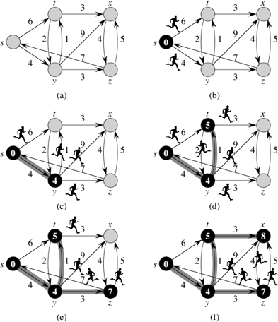
I like to think of Dijkstra's algorithm as a simulation of sending out runners over the graph, starting at the source vertex s. Ideally, the simulation works as follows, though we'll see that Dijkstra's algorithm works slightly differently. It starts by sending out runners from the source vertex to all adjacent vertices. The first time a runner arrives at any vertex, runners immediately leave that vertex, headed to all of its adjacent vertices. Look at part (a) of this figure:
It shows a directed graph with source vertex s and weights next to the edges. Think of the weight of an edge as the number of minutes it would take a runner to traverse the edge.
Part (b) illustrates the start of the simulation, at time 0. At that time, shown inside vertex s, runners leave s and head toward its two adjacent vertices, t and y. The blackened vertex s indicates that we know that s.dist = 0.
Four minutes later, at time 4, the runner to vertex y arrives, shown in part (c). Because this runner is the first to arrive at y, we know that y.dist = 4, and so y is blackened in the figure. The shaded edge (s, y) indicates that the first runner to arrive at vertex y came from vertex s, so that y.pred = s. At time 4, the runner from vertex s to vertex t is still in transit, and runners leave vertex y at time 4, headed toward vertices t, x, and z.
The next event, displayed in part (d), occurs one minute later, at time 5, when the runner from vertex y arrives at vertex t. The runner from s to t has yet to arrive. Because the first runner to arrive at vertex t arrived from vertex y at time 5, we set t.dist to 5 and t.pred to y (indicated by the shaded edge (y, t)). Runners leave vertex t, headed toward vertices x and y at this time.
The runner from vertex s finally arrives at vertex t at time 6, but the runner from vertex y had already arrived there a minute earlier, and so the effort of the runner from s to t went for naught.
At time 7, depicted in part (e), two runners arrive at their destinations. The runner from vertex t to vertex y arrives, but the runner from s to y had already arrived at time 4, and so the simulation forgets about the runner from t to y. At the same time, the runner from y arrives at vertex z. We set z.dist to 7 and z.pred to y, and runners leave vertex z, headed toward vertices s and x.
The next event occurs at time 8, as shown in part (f), when the runner from vertex t arrives at vertex x. We set x.dist to 8 and x.pred to t, and a runner leaves vertex x, heading to vertex z.
At this point, every vertex has had a runner arrive, and the simulation can stop. All runners still in transit will arrive at their destination vertices after some other runner had already arrived. Once every vertex has had a runner arrive, the distvalue for each vertex equals the weight of the shortest path from vertex s and the pred value for each vertex is the predecessor on a shortest path from s.
That was how the simulation proceeds ideally. It relied on the time for a runner to traverse an edge equaling the weight of the edge. Dijkstra's algorithm works slightly differently. It treats all edges the same, so that when it considers the edges leaving a vertex, it processes the adjacent vertices together, and in no particular order. For example, when Dijkstra's algorithm processes the edges leaving vertex s, it declares that y.dist = 4, t.dist = 6, and y.pred and t.pred are both s—so far. When Dijkstra's algorithm later considers the edge (y, t), it decreases the weight of the shortest path to vertex t that it has found so far, so that t.dist goes from 6 to 5 and t.pred switches from s to y.
Dijkstra's algorithm maintains a min-priority queue of vertices, with their dist values as the keys. It repeatedly extracts from the min-priority queue the vertex u with the minimum dist value of all those in the queue, and then it examines all edges leaving u. If v is adjacent to u and taking the edge (u, v) can decrease v's dist value, then we put edge (u, v) into the shortest-path tree (for now, at least), and adjust v.dist and v.pred. Let's denote the weight of edge (u, v) by w(u,v). We can encapsulate what we do for each edge in a relaxation step, with the following pseudocode:
void relax(u, v) {
  if (u.dist + w(u,v) < v.dist) {
    v.dist = u.dist + w(u,v);
    v.pred = u;
  }
}
Whenever a vertex's dist value decreases, the min-priority queue must be adjusted accordingly.
Here is pseudocode for Dijkstra's algorithm, assuming that the source vertex is s:
void dijkstra(s) {
  queue = new PriorityQueue<Vertex>();
  for (each vertex v) {
    v.dist = infinity;  // can use Integer.MAX_VALUE or Double.POSITIVE_INFINITY
    queue.enqueue(v);
    v.pred = null;
  }
  s.dist = 0;

  while (!queue.isEmpty()) {
    u = queue.extractMin();
    for (each vertex v adjacent to u)
      relax(u, v);
  }
}
In the following figure, each part shows the dist value (appearing within each vertex), the pred value (indicated by shaded edges), and the vertices in the min-priority queue (the vertices that are shaded, not blackened) just before each iteration of the while-loop:
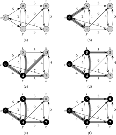
The vertex that is newly blackened in each part of the figure is the vertex chosen as vertex u in in each iteration of the while-loop. In the simulation with runners, once a vertex receives dist and pred values, they cannot change, but here a vertex could receive dist and pred values in one iteration of the while-loop, and a later iteration of the while-loop for some other vertex u could change these values. For example, after edge (y, x) is relaxed in part (c) of the figure, the value of x.dist decreases from ∞ to 13, and x.pred becomes y. The next iteration of the while-loop in (part (d)) relaxes edge (t, x), and x.dist decreases further, to 8, and x.pred becomes t. In the next iteration (part (e)), edge (z, x) is relaxed, but this time x.dist does not change, because its value, 8, is less than z.dist + w(z,x), which equals 12.
When implementing Dijkstra's algorithm, you must take care that the min-priority queue is updated whenever a dist value decreases. For example, the implementation in the textbook uses a HeapAdaptablePriorityQueue, which has a method replaceKey. This method updates the min-priority queue's internal state to reflect the change in a vertex's key. The textbook also relies on a map from Vertex objects to Entry objects, which locate the vertex in the min-priority queue. It's a bit complicated.
You might wonder, since the min-priority queue is going to be implemented by a min-heap, why not just have the Dijkstra's algorithm code keep track of the index of each vertex's index in the array that implements the heap? The problem is that the premise violates our goal of abstraction. Who is to say that a min-heap implements the min-priority queue? In fact, we could just use an unsorted array. Or any other implementation of a min-priority queue. The Dijkstra's algorithm code should know only that it's using a min-priority queue, and not how the min-priority queue is implemented.
How do we know that, at termination (when the min-priority queue is empty because every vertex has been dequeued), v.dist is in fact the shortest-path weight for every vertex v? We rely on a loop invariant argument. We state a property that pertains to a loop, which we call the loop invariant, and we have to show three things about it:
To make our loop invariant a little simpler, let's adopt a notation for all vertices not in the min-priority queue at a given time; we'll call these vertices set S. (This set is sometimes called the "closed set," and vertices still in the queue are called the "open set.") Then here is the loop invariant:
At the start of each iteration of the while-loop,
v.distis the correct shortest-path weight for each vertex v in S.
It's easy to see that the loop invariant holds before the first iteration. At that time, all vertices are in the min-priority queue, and so set S is empty. Therefore, the loop invariant holds vacuously.
Next, let's see how the third part helps. When we exit the loop, the min-priority queue is empty, and so the set S consists of all the vertices. Therefore, every vertex has its correct shortest-path weight.
The hardest part is the second part, where we have to show that each iteration maintains the truth of the loop invariant. We'll give a simplified version of the reasoning. (A formal proof is a bit more involved.) Assume that as we enter an iteration of this loop, all vertices in set S have their correct shortest-path weights in their dist values. Then every edge leaving these vertices has been examined in some relaxation step. Consider the vertex u in the min-priority queue with the lowest dist value. Its dist value can never again decrease. Why not? Because the only edges remaining to be relaxed are edges leaving vertices in the min-priority queue and every vertex in the min-priority queue has a dist value at least as large as u.dist. Since all edge weights are nonnegative, we must have u.dist ≤ v.dist + w(v,u) for every vertex v in the min-priority queue, and so no future relaxation will decrease u.dist. Therefore, u.dist is as low as it can go, and we can extract vertex u from the min-priority queue and relax all edges leaving u. That is, u.dist has its correct shortest-path weight and it is now in set S.
To analyze Dijkstra's algorithm, we'll let n denote the number of vertices and m denote the number of directed edges in the graph (as usual). Each vertex is enqueued once, at the start of the algorithm, and it is never enqueued again, and so there are n enqueue operations. Similarly, each vertex is dequeued once, in some iteration of the while-loop, and because it is never enqueued again, that one time is the only time a vertex is ever dequeued. Hence, there are n dequeue operations. Every edge is relaxed one time, and so there are m relaxation steps and, hence, at most m times that we need to update the min-priority queue because a key has changed. Let's use the generic term decreaseKey for updating the min-priority queue (what the textbook calls replaceKey; I like decreaseKey better, since it's for a min-priority queue). These are the relevant costs: n insert operations, n extractMin operations, and at most m decreaseKey operations. The running time of Dijkstra's algorithm depends on how these operations are implemented.
We can use an unsorted array for the min-priority queue. Each insert and decreaseKey operation takes Θ(1) time. Each extractMin operation takes time O(q), where q is the number of vertices in the min-priority queue at the time. We know that q ≤ n always, and so we can say that each extractMin operation takes O(n) time. But wait—what about when q is small? The way to think about it is to look at the time for all n extractMin operations altogether. You can do the analysis that results in an arithmetic series in n, or you can do it in a simpler way. We have n operations, each taking O(n) time, and so the total time for all extractMin operations is O(n2). If we look at just the first n/2 extractMin operations, each of them has to examine at least n/2 vertices to find the one with the smallest dist value, and so just the first half of the extractMin operations take Ω(n2) time. Hence the total time for the n extractMin operations is Θ(n2), as is the total time for Dijkstra's algorithm.
What if we use a min-heap for the min-priority queue? Now each insert, extractMin, and decreaseKey operation takes O(lg n) time, and so the total time for Dijkstra's algorithm is O((n + m) lg n). If we make the reasonable assumption that m ≥ n − 1 (otherwise, we don't even have a connected graph), then that running time is O(m lg n). That's always better than using an unsorted array, right? No. We say that a graph is dense if m = Θ(n2), that is if on average every vertex has Θ(n) neighbors. In a dense graph, Dijkstra's algorithm runs in time O(n2 lg n), which is worse than using an unsorted array. It is somewhat embarrassing that the "clever" heap is beaten by the "naive" unsorted array.
This embarrassment lasted for decades, until the invention of a data structure called a Fibonacci heap that implements extractMin in O(lg n) amortized time (amortized over all the operations) and insert and decreaseKey in Θ(1) amortized time. With a Fibonacci heap, Dijkstra's algorithm runs in time O(n lg n + m), which is at least as good as using either an unsorted array or a min-heap. Fibonacci heaps are a little tricky to implement, and their hidden constant factors are a little worse than those for binary heaps, but they're not as hard to implement as some people seem to think.
If we are trying to go from Hanover to Boston does it make sense to calculate distances to Montpelier and Burlington?. Of course not. You are going in the "wrong direction." But Dijkstra's algorithm would calculate these distances, because they are closer to Hanover than Boston. How could Dijkstra's algorithm know that looking at Montpelier and Burlington is a waste of time?
If we are looking for the shortest path to a known goal we can use a generalization of Dijkstra's algorithm called A* search to find the shortest path without taking as much time as normal Dijkstra's. The idea is to use an estimate the distance remaining, and to add it to the distance traveled so far to get the key for the city in the PQ. For this case the normal Euclidean distance between Montpelier and Boston would be something like 130 miles. (Figure this Euclidean distance from GPS coordinates of longitude and latitude.) Adding this to the 45 miles from Hanover to Monpelier would give 175 miles. Therefore Boston (whose distance will be 120 miles or so) would come out of the PQ before Montpelier.
Just as in Dijkstra's algorithm, in A* we have a PQ and "closed set" of vertices where we know the best path, so if we discover them again while searching we don't need to deal with them. The second group is the "open set" corresponding to vertices in the PQ. Just as in Dijkstra's when we deleteMin from the PQ we move the corresponding vertex to the closed set and remove it from the PQ and the open set. We then find incident edges and relax them (update an adjacent vertex's current distance if we have found a shorter path). But the key in the PQ is always distance so far plus the estimate of the remaining distance.For this to find the shortest path we need two things. First, the estimate of distance remaining must be admissible. This means that we always underestimate the true remaining distance or get it exactly. Because of the triangle inequality the Euclidean distance is an underestimate of the true travel distance. In fact, the ultimate underestimate of the remaining distance is 0. This leads to normal Dijkstra, because then we take the shortest distance traveled next.
The second requirement is that the cost estimate is monotone. That means that if we extend the path (thus increasing the distance travelled so far), the total estimate is never less that the estimate before we extended the path. This is the generalization of "no negative edges." Our Euclidean distance plus distance so far estimate satisfies this, because if moving to an adjacent vertex increases the distance so far by d it cannot reduce the Euclidean distance by more than d. (It would reduce by exactly d if you were moving directly toward the goal.) Thus the sum will not go down. Using just Euclidean distance (without distance so far) would fail to be monotone, so would not be not guaranteed to give shortest paths.
We often deal with problems where the graph is implicit. Consider a maze. There is an underlying graph - the squares in the maze are the vertices and the edges connect adjacent squares. However, to convert the maze to a graph is more effort than to find the shortest path, because we end up converting parts of the maze that we would never visit. What is worse is a puzzle like the 15-puzzle (15 numbered tiles and a blank in a 4x4 frame, with the tiles able to slide into the blank's position) or Rubic's Cube. Here the size of the implicit graph is potentially enormous. Therefore we create vertex objects as we need them and find adjacencies on the fly. (For the 15-puzzle two configurations are adjacent if they differ by sliding one tile into the blank position and for Rubic's cube two configurations are adjacent if they differ by a twist.)
Suppose we want to find paths in a maze. We can used DFS, but this can lead to very long paths. (Demo maze5 in the Maze program.) BFS will guarantee finding the shortest path, but this can be very slow. We can improve on DFS by using a heuristic, e.g. the L1 (Manhattan) distance from where we are to the target square. (This means adding the x difference to the y difference between the two squares.) If we use a PQ based on this distance we will tend to "zoom in" on the target. However, this will not guarantee a shortest path. (Again demo the maze program.) Can we do better? Yes. Using A* search we can find the shortest path without taking as much time as BFS. The idea is to add a heuristic like the L1 distance to estimate the distance remaining. For our maze the L1 distance is an admissible estimate - we move either horizontally or vertically in each step, so the number of steps needed is at least the L1 distance. Note we could also have used the Euclidean distance. That would be a bigger underestimate, because we the Euclidean distance will usually be smaller than the L1 distance and will never be larger. Demo on maze5, showing that the square where the paths meet will be discovered from the right first, but will be eventually included in the path from the left.
Note that using a remaining distance estimate of 0 gives BFS on the implicit maze graph, because the shortest path is always expanded next.
Look at how the maze program implements this via Sequencers (generalized priority queues) and SequenceItems (to keep track of squares in the matrix and the path so far). The StackSequencer and QueueSequencer use a stack and queue respectively to add and get next items. The DistSequencer uses a priority queue, where the priority is the L1 distance to the target. This distance gets saved in the key field in the PQSequenceItem and is used when comparing PQSequenceItems in the priority queue.
The AStarSequencer keeps track of the open set via a map from SequenceItems to Entries in the PQ, so that when we find a shorter distance we can find and update the approprite PQ Entry. It also has an AdaptablePriorityQueue to allow the value of an entry's key to be changed when relaxation finds a better path. The AStarSequenceItem has an instance variable to hold the path length and a method get it, because that is part of the estimate. Note that SequenceItems are equal if the row and column positions are equal. Note that we overrode hashCode to make the hashCodes of equal items equal.
The code for the Maze solver is in:
MazeSrc.zip.