We continue looking at methods in SentinelDLL.java. We've already seen the constructor, clear, toString, add, remove, and contains.
The remaining list methods are really easy. Note that the later methods use the isEmpty, hasCurrent, and hasNext predicates rather than just doing the tests directly. Accessing the linked list through these methods makes changing the representation easier.
isEmpty returns true if and only if the only list element is the sentinel. That is the case precisely when the sentinel references itself.hasCurrent returns true if and only if there is a current element. That is the case precisely when current does not reference the sentinel.hasNext returns true if there are both a current element and another element after the current element.getFirst sets the current reference to the first element in the list and returns the data in the first element. If the list is empty, then current must reference the sentinel, and its data must be null, and so getFirst returns null when the list is empty.getLast is like getFirst except that it sets current to reference the last element in the list and return its data.addFirst adds a new element at the head of the list and makes it the current element.addLast adds a new element at the tail of the list and makes it the current element.next moves current to current.next and returns the data in that next element. It returns null if there is no next element.get returns the data in the current element, or null if there is no current element.set assigns to the current element, printing an error message to System.err if there is no current element.All of the above methods are in the CS10LinkedList interface. In addition, the SentinelDLL class contains two methods (other than the constructor) that are not in the CS10LinkedList interface:
previous moves current to current.previous and returns the data in that previous element. It returns null if there is no previous element.hasNext returns true if there are both a current element and another element before the current element.SentinelDLL classWe can use the ListTest.java program to test the SentinelDLL class. You can use the debugger to examine the linked list if you like.
Notice that to declare and create the linked list, we specify the type that will be stored in the list. Here, it's a String:
CS10LinkedList<String> theList = new SentinelDLL<String>();Because theList is declared as a reference to the interface CS10LinkedList, we cannot call the previous or hasPrevious methods in this driver.
Although doubly linked circular linked lists with sentinels are the easiest linked lists to implement, they can take a lot of space. There are two references (next and previous) in each element, plus the sentinel node. Some applications create a huge numbers of very short linked lists. (One is hashing, which we'll see later in this course.) In such situations, the extra reference in each node and the extra node for the sentinel can take substantial space.
The code for singly linked lists has more special cases than the code for circular, doubly linked lists with a sentinel, and the time to remove an element in a singly linked list is proportional to the length of the list in the worst case rather than the constant time it takes in a circular, doubly linked list with a sentinel.
The SLL class in SLL.java implements the CS10LinkedList interface with a generic type T, just as the SentinelDLL class does. A singly linked list, as implemented in the SLL class, has two structural differences from a circular, doubly linked list with a sentinel:
Each Element object in a singly linked list has no backward (previous) reference; the only navigational aid is a forward (next) reference.
There is no sentinel, nor does the list have a circular structure. Instead, the SLL class maintains references head to the first element on the list and tail to the last element on the list.
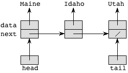
A singly linked list with Maine, Idaho, and Utah would look like

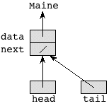
A singly linked list with only one element would look like
And an empty singly linked list looks like

The file SLL.java contains the class definitions for Element and SLL for a singly linked list. These declarations are similar to those for circular, doubly linked lists with a sentinel. As before, Element class is a private inner class, and all method declarations are the same. The only difference is in the instance data. We can use the same ListTest.java driver to test the singly linked list class, as long as we change the line creating the list to read
CSLinkedList<String> theList = new SLL<String>();We can make a similar change to ListTraverse.java to traverse a singly linked list from outside the class.
Let's examine the List methods in SLL.java for singly linked lists. We will highlight those that differ from those for circular, doubly linked lists with a sentinel.
The clear method, which is called by the SLL constructor as well as being publicly available, makes an empty list by setting all instance variables (head, tail, and current) to null.
As before, the add method places a new Element object after the one that current references. Without a special case, however, there would be no way to add an element as the new head of the list, since there is no sentinel to put a new element after. Therefore, if current is null, then we add the new element as the new list head.
The code, therefore, has two cases, depending on whether current is null. If it is, we have to make the new element reference what head was referencing and then make head reference the new element. Otherwise, we make the new element reference what the current element is referencing and then make current reference the new element. If the new element is added after the last element on the list, we also have to update tail to reference the new element.
Compare this code to the add code for a circular, doubly linked list with a sentinel. Although there is only one directional link to maintain for a singly linked list, the code has more cases and is more complex. For either implementation, however, adding an element takes constant time.
As mentioned, removing an element from a singly linked list takes time proportional to the length of the list in the worst case—in other words, time that is linear in the length of the list— which is worse than the constant time required for a circular, doubly linked list with a sentinel. Why does it take linear time, rather than constant time? The reason is that the previous reference in a doubly linked list really helps. In order to splice out the current element, we need to know its predecessor in the list, because we have to set the next instance variable of the predecessor to the value of current.next. With the previous reference, we can easily find the predecessor in constant time. With only next references available, the only way we have to determine an element's predecessor is to traverse the list from the beginning until we find an element whose next value references the element we want to splice out. And that traversal takes linear time in the worst case, which is when the element to be removed is at or near the end of the list.
The remove method first checks that current, which references the Element object to be removed, is non-null. If current is null, we print an error message and return. Normally, current is non-null, and the remove method finds the predecessor pred of the element that current references. Even this search for the predecessor has two cases, depending on whether the element to be removed is the first one in the list. If we are removing the first element, then we set pred to null and update head. Otherwise, we have to perform a linear search, stopping when pred.next references the same element as current; once this happens, we know that pred is indeed the predecessor of the current element. (There is also some "defensive coding," just in case we simply do not find an element pred such that pred.next references the same element as current. We do not expect this to ever happen, but if it does, we have found a grave error and so we print an error message and return.) Assuming that we find a correct predecessor, we splice out the current element. We also have to update tail if we are removing the last element of the list.
The bottom line is that, compared with the remove code for a circular, doubly linked list with a sentinel, the remove code for a singly linked list is more complex, has more possibilities for error, and can take longer.
toString for a listThe toString for a singly linked list is similar to how we print a circular, doubly linked list with a sentinel, except that now we start from head rather than sentinel.next and that the termination condition is not whether we come back to the sentinel but rather whether the reference we have is null. The for-loop header, therefore, is
for (x = head; x != null; x = x.next)The contains method for a singly linked list is perhaps a little shorter than for a circular, doubly linked list with a sentinel, because now we do not replace the object reference in the sentinel. The for-loop header, therefore, becomes a little more complicated. We have to check whether we have run off the end of the list (which we did not have to do when we stored a reference to the object being searched for in the sentinel) and then, once we know we have not run off the end, whether the element we are looking at equals the object we want. The bodyless for-loop is
for (x = head; x != null && !x.data.equals(obj); x = x.next)
  ;
Although the code surrounding the for-loop simplifies with a singly linked list, the loop itself is cleaner for the circular, doubly linked list with a sentinel. Either way, it takes linear time in the worst case.
isEmpty is easy, but slightly different from the version for a circular, doubly linked list with a sentinel. We simply return a boolean that indicates whether head is null.hasCurrent returns true if and only if the there is a current element. We simply return a boolean indicating whether current is not null.hasNext checks to see whether there is a current element and whether the next field of the current element is null rather than seeing if it is the sentinel.getFirst is different, as it sets current to head.getLast changes, too, setting current to tail.addFirst and addLast are similar to a circular, doubly linked list with a sentinel. However, addLast has to deal with an empty list separately.get is unchanged.next is identical to the version in the doubly linked list. (This is an advantage of calling hasNext rather than doing the test directly in this method.)previous and hasPrevious methods. We are not required to, because they're not in the CS10LinkedList interface.It is also possible to have a dummy list head, even if the list is not circular. If we do so, we can eliminate some special cases, because adding at the head becomes more similar to adding anywhere else. (Instead of changing the head you update a next field.) It is also possible to have current reference the element before the element that it actually indicates, so that removal can be done in constant time. It takes a while to get used to having current reference the element before the one that is actually "current."
It is also possible to have a circular singly linked list, either with or without a sentinel.
You have probably seen big-Oh notation before, but it's certainly worthwhile to recap it. In addition, we'll see a couple of other related asymptotic notations. Chapter 4 of the textbook covers this material as well.
Remember back to linear search and binary search. Both are algorithms to search for a value in an array with n elements. Linear search marches through the array, from index 0 through the highest index, until either the value is found in the array or we run off the end of the array. Binary search, which requires the array to be sorted, repeatedly discards half of the remaining array from consideration, considering subarrays of size n, n/2, n/4, n/8, …, 1, 0 until either the value is found in the array or the size of the remaining subarray under consideration is 0.
The worst case for linear search arises when the value being searched for is not present in the array. The algorithm examines all n positions in the array. If each test takes a constant amount of time—that is, the time per test is a constant, independent of n—then linear search takes time c1n + c2, for some constants c1 and c2. The additive term c2 reflects the work done before and after the main loop of linear search. Binary search, on the other hand, takes c3 log2 n + c4 time in the worst case, for some constants c3 and c4. (Recall that when we repeatedly halve the size of the remaining array, after at most log2 n + 1 halvings, we've gotten the size down to 1.) Base-2 logarithms arise so frequently in computer science that we have a notation for them: lg n = log2 n.
Where linear search has a linear term, binary search has a logarithmic term. Recall that lg n grows much more slowly than n; for example, when n = 1,000,000,000 (a billion), lg n is approximately 30.
If we consider only the leading terms and ignore the coefficients for running times, we can say that in the worst case, linear search's running time "grows like" n and binary search's running time "grows like" lg n. This notion of "grows like" is the essence of the running time. Computer scientists use it so frequently that we have a special notation for it: "big-Oh" notation, which we write as "O-notation."
For example, the running time of linear search is always at most some linear function of the input size n. Ignoring the coefficients and low-order terms, we write that the running time of linear search is O(n). You can read the O-notation as "order." In other words, O(n) is read as "order n." You'll also hear it spoken as "big-Oh of n" or even just "Oh of n."
Similarly, the running time of binary search is always at most some logarithmic function of the input size n. Again ignoring the coefficients and low-order terms, we write that the running time of binary search is O(lg n), which we would say as "order log n," "big-Oh of log n," or "Oh of log n."
In fact, within our O-notation, if the base of a logarithm is a constant (such as 2), then it doesn't really matter. That's because of the formula
$\displaystyle\log_a n = \frac{\log_b n}{\log_b a}$
for all positive real numbers a, b, and c. In other words, if we compare loga n and logb n, they differ by a factor of logb a, and this factor is a constant if a and b are constants. Therefore, even when we use the "lg" notation within O-notation, it's irrelevant that we're really using base-2 logarithms.
O-notation is used for what we call "asymptotic upper bounds." By "asymptotic" we mean "as the argument (n) gets large." By "upper bound" we mean that O-notation gives us a bound from above on how high the rate of growth is.
Here's the technical definition of O-notation, which will underscore both the "asymptotic" and "upper-bound" notions:
A running time is O(n) if there exist positive constants n0 and c such that for all problem sizes n ≥ n0, the running time for a problem of size n is at most cn.
Here's a helpful picture:
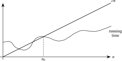
The "asymptotic" part comes from our requirement that we care only about what happens at or to the right of n0, i.e., when n is large. The "upper bound" part comes from the running time being at most cn. The running time can be less than cn, and it can even be a lot less. What we require is that there exists some constant c such that for sufficiently large n, the running time is bounded from above by cn.
For an arbitrary function f(n), which is not necessarily linear, we extend our technical definition:
A running time is O(f(n)) if there exist positive constants n0 and c such that for all problem sizes n ≥ n0, the running time for a problem of size n is at most c f(n).
A picture:
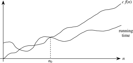
Now we require that there exists some constant c such that for sufficiently large n, the running time is bounded from above by c f(n)
Actually, O-notation applies to functions, not just to running times. But since our running times will be expressed as functions of the input size n, we can express running times using O-notation.
In general, we want as slow a rate of growth as possible, since if the running time grows slowly, that means that the algorithm is relatively fast for larger problem sizes.
We usually focus on the worst case running time, for several reasons:
You might think that it would make sense to focus on the "average case" rather than the worst case, which is exceptional. And sometimes we do focus on the average case. But often it makes little sense. First, you have to determine just what is the average case for the problem at hand. Suppose we're searching. In some situations, you find what you're looking for early. For example, a video database will put the titles most often viewed where a search will find them quickly. In some situations, you find what you're looking for on average halfway through all the data…for example, a linear search with all search values equally likely. In some situations, you usually don't find what you're looking for…like at Radio Shack.
It is also often true that the average case is about as bad as the worst case. Because the worst case is usually easier to identify than the average case, we focus on the worst case.
Computer scientists use notations analogous to O-notation for "asymptotic lower bounds" (i.e., the running time grows at least this fast) and "asymptotically tight bounds" (i.e., the running time is within a constant factor of some function). We use Ω-notation (that's the Greek leter "omega") to say that the function grows "at least this fast." It is almost the same as Big-Oh notation, except that is has an "at least" instead of an "at most":
A running time is Ω(f(n)) if there exist positive constants n0 and c such that for all problem sizes n ≥ n0, the running time for a problem of size n is at least c f(n).
We use Θ-notation (that's the Greek letter "theta") for asymptotically tight bounds:
A running time is Θ(f(n)) if there exist positive constants n0, c1, and c2 such that for all problem sizes n ≥ n0, the running time for a problem of size n is at least c1 f(n) and at most c2 f(n).
Pictorially,
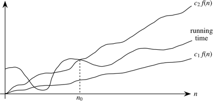
In other words, with Θ-notation, for sufficiently large problem sizes, we have nailed the running time to within a constant factor. As with O-notation, we can ignore low-order terms and constant coefficients in Θ-notation.
Note that Θ-notation subsumes O-notation in that
If a running time is Θ(f(n)), then it is also O(f(n)).
The converse (O(f(n)) implies Θ(f(n))) does not necessarily hold.
The general term that we use for O-notation, Θ-notation, and Ω-notation is asymptotic notation.
Asymptotic notations provide ways to characterize the rate of growth of a function f(n). For our purposes, the function f(n) describes the running time of an algorithm, but it really could be any old function. Asymptotic notation describes what happens as n gets large; we don't care about small values of n. We use O-notation to bound the rate of growth from above to within a constant factor, and we use Θ-notation to bound the rate of growth to within constant factors from both above and below. (We won't use Ω-notation much in this course.)
We need to understand when we can apply each asymptotic notation. For example, in the worst case, linear search runs in time proportional to the input size n; we can say that linear search's worst-case running time is Θ(n). It would also be correct, but slightly less precise, to say that linear search's worst-case running time is O(n). Because in the best case, linear search finds what it's looking for in the first array position it checks, we cannot say that linear search's running time is Θ(n) in all cases. But we can say that linear search's running time is O(n) in all cases, since it never takes longer than some constant times the input size n.
Although the definitions of O-notation an Θ-notation may seem a bit daunting, these notations actually make our lives easier in practice. There are two ways in which they simplify our lives.
I won't go through the math that follows in class. You may read it, in the context of the formal definitions of O-notation and Θ-notation, if you wish. For now, the main thing is to get comfortable with the ways that asymptotic notation makes working with a function's rate of growth easier.
Constant multiplicative factors are "absorbed" by the multiplicative constants in O-notation (c) and Θ-notation (c1 and c2). For example, the function 1000 n2 is Θ(n2) since we can choose both c1 and c2 to be 1000.
Although we may care about constant multiplicative factors in practice, we focus on the rate of growth when we analyze algorithms, and the constant factors don't matter. Asymptotic notation is a great way to suppress constant factors.
When we add or subtract low-order terms, they disappear when using asymptotic notation. For example, consider the function n2 + 1000 n. I claim that this function is Θ(n2). Clearly, if I choose c1 = 1, then I have n2 + 1000 n ≥ c1 n2, and so this side of the inequality is taken care of.
The other side is a bit tougher. I need to find a constant c2 such that for sufficiently large n, I'll get that n2 + 1000 n ≤ c2 n2. Subtracting n2 from both sides gives 1000 n ≤ c2 n2 − n2 = (c2 − 1) n2. Dividing both sides by (c2 − 1) n gives $\displaystyle \frac{1000}{c_2 - 1} \leq n$. Now I have some flexibility, which I'll use as follows. I pick c2 = 2, so that the inequality becomes $\displaystyle \frac{1000}{2-1} \leq n$, or 1000 ≤ n. Now I'm in good shape, because I have shown that if I choose n0 = 1000 and c2 = 2, then for all n ≥ n0, I have 1000 ≤ n, which we saw is equivalent to n2 + 1000 n ≤ c2 n2.
The point of this example is to show that adding or subtracting low-order terms just changes the n0 that we use. In our practical use of asymptotic notation, we can just drop low-order terms.
In combination, constant factors and low-order terms don't matter. If we see a function like 1000 n2 − 200 n, we can ignore the low-order term 200 n and the constant factor 1000, and therefore we can say that 1000 n2 − 200 n is Θ(n2).
As we have seen, we use O-notation for asymptotic upper bounds and Θ-notation for asymptotically tight bounds. Θ-notation is more precise than O-notation. Therefore, we prefer to use Θ-notation whenever it's appropriate to do so.
We shall see times, however, in which we cannot say that a running time is tight to within a constant factor both above and below. Sometimes, we can bound a running time only from above. In other words, we might only be able to say that the running time is no worse than a certain function of n, but it might be better. In such cases, we'll have to use O-notation, which is perfect for such situations.
Let's consider the following problem:
Suppose you have a program that runs the selection sort algorithm, which takes Θ(n2) time to sort n items. Suppose further that, when given an input array of 10,000 items, this selection sort program takes 0.1 seconds. How long would the program take to sort an array of 1,000,000 items? Would you wait for it? Would you go get coffee? Go to dinner? Go to sleep?
Here's how we can analyze this problem. First, we won't worry about low-order terms, especially because we're working with large problem sizes. So we can figure that selection sort takes approximately cn2 seconds to sort. When n = 10,000, we have that cn2 = 100,000,000 c = 0.1 seconds. Dividing both sides by 100,000,000, we get that c = 10 − 9.
So now we can determine how long it takes to sort when n = 1,000,000. Here, n2 = 1012, and so cn2 = 10 − 9 × 1012 = 1000 seconds, or $16\frac{2}{3}$ minutes. Unless you eat very fast, you have time for coffee but not for dinner. (Or you have time for a power nap.)
Let's generalize this idea to other running times. Suppose that the running time of a program is Θ(nk) for some constant k. What happens when the input size changes by a factor of p, so that the input size goes from n to pn? Again, let's ignore the low-order terms and say that the running time is approximately f(n) = cnk for an input of size n. Then f(pn) = c(pn)k = pk cnk = pk f(n). So the running time changes by a factor of pk. In our previous problem, k = 2 and p = 100, and so the running time increases by a factor of 1002 = 10,000, from 0.1 seconds to 1000 seconds.
Now let's suppose that instead of selection sort, we were running merge sort, whose running time is Θ(n lg n). As before, we ignore low-order terms and approximate the running time of merge sort as f(n) = cn lg n. We have that lg 10,000 is approximately 13.29, and so if the running time of merge sort is 0.1 seconds, then we have c × 10,000 × 13.29 = 0.1, and so c = 0.1/(10,000 × 13.29) = 7.52 × 10 − 7. When n = 1,000,000, we have that lg n is approximately 19.93, and so f(n) = (7.52 × 10 − 7) × 1,000,000 × 19.93 = 14.99 seconds. That's enough time to take a sip of coffee, but not much more.