Last time, we started to look at expression trees. We saw the files Expression.java, Constant.java, and Variable.java, plus some exceptions that can be thrown by methods of the Variable class (in MultiplyDefinedVariableException.java, UndefinedVariableException.java, and UnassignedVariableException.java).
The classes in Sum.java, Difference.java, Product.java, and Quotient.java all perform eval by evaluating their operands and performing an operation on them. The only difference is the operator. Therefore, we have an abstract class in BinaryOp.java that has the template for evaluating a binary expression and another template for toString. These templates call abstract functions doOperation and getOperation, repectively. (The latter returns a String representation of the operator). It also has accessor methods to get the first or second expression.
Notice that evaluating an expression is really a postorder traversal of the expression tree. To evaluate a BinaryOp, first evaluate its two subtrees, and then apply the appropriate binary operator to the results of evaluating the subtrees.
Let's look at the Sum class more carefully. It provides the necessary two methods, which are fairly trivial. It supplies its deriv method, which adds the derivatives of its operands. But the interesting thing is Sum.make. Here we see the power of a factory method. It tries to simplify the expression. If the two expressions it is adding are constants, it adds them to get a new constant. If either operand is 0 it returns the other. So in three of the four cases it does not even create a Sum object! The other three operations are similar in how they try to simplify the resulting expression in their make methods.
Finally, look at the driver in ExpressionDriver.java. After the main method, we have several static wrapper methods. They alleviate the need to call the static methods in the above classes with the name of the class. We also use method names plus, minus, times, and over instead of the class names Sum, Difference, Product, and Quotient. In that way, we can construct the expression tree above using lines of code such as
Variable xVar = define("x", 2.0);
Variable yVar = define("y", 6.0);

Expression first = plus(constant(17.5), over(constant(5.0), xVar));
Expression second = minus(yVar, constant(4.0));
Expression third = times(first, second);
Or we can replace the last three lines by
Expression fourth = times(plus(constant(17.5), over(constant(5.0), xVar)),
    minus(yVar, constant(4.0)));
The driver also verifies that the three exceptions work correctly.
We often need to model entities that have connections between them. For example, we might want to know whether two people are friends. If we can identify a group of people all of whom are friends with each other that might tell us something about these people; for example, they might all be members of the same Greek house, or that they might constitute a terrorist cell.
For another example of entities with connections, think of a road map. Each intersection is an entity, and a connection is a road going between two intersections.
Here's another example. When you get dressed, there are some articles of clothing that you must put on before other articles, such as socks before shoes. But there are also some articles for which the order that you don them does not matter, such as socks and a shirt. So we can say that there's a connection between two articles of clothing if you have to put on one before the other.
Sometimes we need to know more than just that there's a connection; there's some quantitative aspect of the connection that's important. For a road map, we might care not only that a road connects two intersections, but also about the length of the road. For another example, we might want to know, for any pair of world currencies, the exchange rate from one to the other.
Many years ago, mathematicians devised a nice way to model situations with many entities and relationships between pairs of entities: a graph. A graph consists of vertices (singular: vertex) connected by edges. Each edge connects one vertex to some other vertex. A vertex may have edges to zero, one, or many other vertices. Think of each vertex as representing an entity and each edge as a connection.
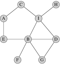
Here's a simple graph with 9 vertices and 11 edges:

Each vertex in this particular graph is labeled by a letter, though in general we can label vertices however we like, including with no label at all. Just to take an example, vertex A has two edges: one to vertex C and one to vertex E.
In some situations, we want directed edges, where we care about the edge going from one vertex to another vertex. Directed edges work well in the example about getting dressed, where an edge from a vertex for article X to a vertex for article Y indicates that you have to don X before Y. In other situations, such as the graph drawn above, the edges are undirected. Because the friendship relation is symmetric, if we consider a graph in which vertices represent people and an edge between persons X and Y indicates that X and Y are friends, this graph would have undirected edges. A graph with undirected edges is an undirected graph, and a graph with directed edges is a directed graph. Then again, a graph of who loves whom should be directed, since love is not always reciprocated. We can always emulate an undirected edge between vertices x and y with directed edges from x to y and from y to x.
When we put a numeric value on an edge, say to indicate the length of a road, we call that an edge weight, "weight" being a generic term for the quantity that we care about. (Unless you're a civil engineer building elevated highways, you probably don't care how much a road actually weighs.) Edges can be weighted or unweighted in either directed or undirected graphs.
You might sometimes hear other names for these structures. Graphs are sometimes called networks, vertices are sometimes called nodes (you might recall that when I drew trees, I used the term), and edges are sometimes referred to as links or arcs.
A few more easy definitions. In mathematics, we write the name of an edge from vertex x to vertex y as (x, y). If the edge is undirected, then (y, x) is the same edge as (x, y), but not if the edge is directed. In an undirected graph, we say that the edge (x, y) is incident on vertices x and y, and we also say that x and y are adjacent to each other, and they are neighbors. In the above graph, vertices D and G are adjacent and edge (D, G) is incident on both of them. In a directed graph, edge (x, y) leaves x and enters y, and y is adjacent to x (but x is not adjacent to y unless the edge (y, x) is also present). The number of edges incident on a vertex in an undirected graph is the degree of the vertex. In the above graph, the degree of vertex B is 5. In a directed graph, the number of edges leaving a vertex is its out-degree and the number of edges entering a vertex is its in-degree.
If we can get from vertex x to vertex y by following a sequence of edges, we say that the vertices along the way, including x and y, form a path from x to y. A simple path is a path with no repeated vertices. The length of the path is the number of edges on the path. In the above graph, one path from vertex D to vertex A contains the vertices, D, I, C, A, with 3 edges; another path contains the vertices D, G, B, E, A, with 4 edges. Note that there is always a path of length 0 from any vertex to itself. A path from a vertex to itself containing at least one edge, and with all edges distinct, is a cycle. In the above graph, one cycle contains the vertices A, E, B, G, D, I, C, A; another cycle contains the vertices A, E, B, I, C, A. An undirected graph is connected if all pairs of vertices have some path between them.
We'll focus on undirected graphs in CS 10, but we'll also occasionally discuss directed graphs.
We can choose from among a few ways to represent a graph. Some ways are better for certain purposes than other ways. It's convenient to have a standard notation for the numbers of vertices and edges in a graph, and so we'll always use n for the number of vertices and m for the number of edges (either directed or undirected). It is often convenient to number vertices, and when we do, we number them from 0 to n − 1.
One simple representation is just an array of m edges, which we call an edge list. To represent an edge, we just give the numbers of the two vertices it's incident on. Each edge in the array is some object that includes the two vertex numbers. If the edge has a weight, the edge object also includes the weight.
Edge lists are simple, and they take only Θ(m) space, but if we want to find whether the graph contains a particular edge, we have to search through the array. If the edges appear in the array in no particular order, that's a linear search through m edges, taking Θ(m) time in the worst case. Question to think about: How can you organize an edge list to make searching for a particular edge take O(lg m) time? The answer is a little tricky.
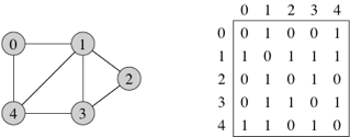
For a graph with n vertices, an adjacency matrix is an n × n matrix of 0s and 1s, where the entry in row i and column j is 1 if and only if the edge (i, j) is in the graph. (Recall that we can represent an n × n matrix by an n-element array in which each entry references an array of n numbers.) If you want to indicate an edge weight, put it in the row i, column j entry, and reserve a special value (for example, if a super-high weight indicates an absent edge, you can use Double.POSITIVE_INFINITY or Integer.MAX_VALUE) to indicate an absent edge. Here's a unweighted, undirected graph and its adjacency matrix:

With an adjacency matrix, we can find out whether an edge is present in constant time, by just looking up the corresponding entry in the matrix. So what's the disadvantage of an adjacency matrix? Two things, actually. First, it takes Θ(n2) space, even if the graph is sparse: relatively few edges. In other words, for a sparse graph, the adjacency matrix is mostly 0s, and we use lots of space to represent only a few edges. Second, if you want to find out which vertices are adjacent to a given vertex i, you have to look at all n entries in row i, taking Θ(n) time, even if only a small number of vertices are adjacent to vertex i.
For an undirected graph, the adjacency matrix is symmetric: the row i, column j entry is 1 if and only if the row j, column i entry is 1. For a directed graph, the adjacency matrix need not be symmetric.
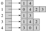
Representing a graph with adjacency lists combines adjacency matrices with edge lists. For each vertex x, store a list of the vertices adjacent to it. We typically have an array of n adjacency lists, one adjacency list per vertex. We can store an adjacency list with an array (if we don't plan to insert or remove adjacent vertices) or a linked list (if we expect to insert or remove adjacent vertices). Here's an adjacency-list representation of the graph from above, using arrays:

We can get to each vertex's adjacency list in O(1) time, because we just have to index into the array of adjacency lists. To find out whether an edge (x, y) is present in the graph, we go to x's adjacency list in O(1) time and then look for y in x's adjacency list. How long does that take in the worst case? Θ(d), where d is the degree of x, because that's how long x's adjacency list is. The degree of x could be as high as n − 1 (if x is adjacent to all other n − 1 vertices) or as low as 0 (if x is isolated, with no incident edges). In an undirected graph, y is in x's adjacency list if and only if x is in y's adjacency list. If the graph is weighted, then each element in each adjacency list includes the edge weight.
How much space do adjacency lists take? We have n lists, and although each list could have as many as n − 1 vertices, in total the adjacency lists for an undirected graph contain 2m items. Why 2m? Each edge (x, y) appears exactly twice in the adjacency lists, once in x's list and once in y's list, and there are m edges. For a directed graph, the adjacency lists contain a total of m items, one item per directed edge.
The textbook has another representation, the adjacency map, which the authors claim combines the best of adjacency lists and adjacency matrices. Instead of using an array or a linked list for each adjacency list, they use a map, implemented by a hash table. For a directed graph, each vertex has a hash table for its entering edges and a different hash table for its leaving edges, so that a directed graph has 2n hash tables altogether. For an undirected graph, each vertex has just one hash table, for a total of n hash tables. Now you can determine whether an edge (u, v) is present in O(1) expected time by going to u's hash table and, in O(1) expected time, seeing whether u's hash table has an entry for v.
The adjacency map representation is implemented in AdjacencyMapGraph.java. The AdjacencyMapGraph class is part of a large package called net.datastructures that is associated with the textbook; I've created a zip file of the entire package. To use it within an Eclipse project after you've uncompressed, first select the src folder within the project in the Package Explorer pane. Then choose File -> New -> Package, and enter net.datastructures for the package name. Then you can drag the 51 java files in the uncompressed folder into net.datastructures in your Eclipse project. If you're going to use any of these classes, then you'll need to have the line
import net.datastructures.*;in your Java file.
You need to use at least two other classes in net.datastructures if you're going to use AdjacencyMapGraph. The Vertex and Edge classes take generic types that say what information you're storing in a vertex or edge.
Here is a list of the methods in the AdjacencyMapGraph class. Some of them throw an IllegalArgumentException if given a bad parameter, such as a vertex or edge not actually in the graph.
true) or undirected (false).Vertex<V> insertVertex(V element) inserts a vertex into the graph and returns a reference to its Vertex object. The parameter element is the information you want to store with the vertex, such as its name (in which case, the generic type V would be String).Edge<E> insertEdge(Vertex<V> u, Vertex<V> v, E element) throws IllegalArgumentException inserts an edge into the graph, once you have created its two vertices. The parameter element is the information you want to store with the edge. If there is already an edge (u, v) in the graph, insertEdge throws an IllegalArgumentException.Iterable<Edge<E>> incomingEdges(Vertex<V> v) throws IllegalArgumentException returns an iterator that goes through all the edges that enter vertex v.Iterable<Edge<E>> outgoingEdges(Vertex<V> v) throws IllegalArgumentException returns an iterator that goes through all the edges that leave vertex v.Vertex<V> opposite(Vertex<V> v, Edge<E> e) throws IllegalArgumentException returns the vertex at the other end of edge e from vertex v.Edge<E> getEdge(Vertex<V> u, Vertex<V> v) throws IllegalArgumentException returns the edge (u, v), or null if the graph contains no such edge.Vertex<V>[] endVertices(Edge<E> e) throws IllegalArgumentException returns a two-element array containing the vertices that edge e is incident on.void removeVertex(Vertex<V> v) throws IllegalArgumentException removes vertex v and all its incident edges from the graph.void removeEdge(Edge<E> e) throws IllegalArgumentException removes edge e from the graph.Iterable<Vertex<V>> vertices() returns an iterator that goes through all the vertices in the graph.Iterable<Edge<E>> edges() returns an iterator that goes through all the edges in the graph.int numVertices() returns the number of vertices in the graph.int numEdges() returns the number of edges in the graph.int inDegree(Vertex<V> v) throws IllegalArgumentException returns the in-degree of vertex v.int outDegree(Vertex<V> v) throws IllegalArgumentException returns the out-degree of vertex v.String toString() returns, as usual, the string representation of the graph. Don't call toString in your code, but it's useful when debugging.I have created a subclass of AdjacencyMapGraph in NamedAdjacencyMapGraph.java. The NamedAdjacencyMapGraph class does everything that an AdjacencyMapGraph does, and it also maintains a map from vertex names (or whatever information you store with a vertex) to the Vertex object. In addition to the methods of AdjacencyMapGraph, it provides the following:
Vertex<V> getVertex(V name) returns the Vertex object corresponding to the name in the parameter, or null if there is no vertex with that name.boolean vertexInGraph(V name) returns a boolean indicating whether the graph contains a vertex with the name in the parameter.Edge<E> insertEdge(V uName, V vName, E element) throws IllegalArgumentException inserts an edge whose vertices have the names uName and vName into the graph. Like the insertEdge method of AdjacencyMapGraph, it throws an IllegalArgumentException if there is already an edge (u, v) in the graph.Edge<E> getEdge(V uName, V vName) throws IllegalArgumentException returns the edge whose endpoints are named by uName and vName, or null if the graph contains no such edge.I find NamedAdjacencyMapGraph to be a convenient way to access vertices and their edges by the names of the vertices, rather than by the Vertex objects.