PS-5
The goal of this problem set is to build a personal digital assistant named "Sudi". Okay, we'll stop short of that, but we will tackle part of the speech understanding problem that a digital assistant such as Sudi would have to handle.
Background
A part of speech (POS) tagger labels each word in a sentence with its part of speech (noun, verb, etc.). For example:
I fish
Will eats the fish
Will you cook the fish
One cook uses a saw
A saw has many uses
You saw me color a fish
Jobs wore one color
The jobs were mine
The mine has many fish
You can cook many
===>
I/PRO fish/V
Will/NP eats/V the/DET fish/N
Will/MOD you/PRO cook/V the/DET fish/N
One/DET cook/N uses/VD a/DET saw/N
A/DET saw/N has/V many/DET uses/N
You/PRO saw/VD me/PRO color/V a/DET fish/N
Jobs/NP wore/VD one/DET color/N
The/DET jobs/N were/VD mine/PRO
The/DET mine/N has/V many/DET fish/N
You/PRO can/MOD cook/V many/PRO
where the tags are after the slashes, indicating e.g., that in the first sentence "I" is a pronoun (PRO), "fish" is a verb (V); in the second sentence, "Will" is a proper noun (NP), "eats" a verb, "the" a determiner (DET), and "fish" a noun (N). If you notice, I purposely constructed these somewhat strange sentences so that the same word serves as a different part of speech in different places ("fish" as both a verb and a noun, "Will" as both a person's name and the future tense modifier, "saw" as both a past tense verb and a tool, etc.). A good tagger makes use of the context to disambiguate the possibilities and determine the correct label. The tagging is in turn a core part of having a "Sudi" understand what a sentence means and how to respond.
The tags that we'll use for this problem set are taken from the book Natural Language Processing with Python:
| Tag | Meaning | Examples |
|---|---|---|
| ADJ | adjective | new, good, high, special, big, local |
| ADV | adverb | really, already, still, early, now |
| CNJ | conjunction | and, or, but, if, while, although |
| DET | determiner | the, a, some, most, every, no |
| EX | existential | there, there's |
| FW | foreign word | dolce, ersatz, esprit, quo, maitre |
| MOD | modal verb | will, can, would, may, must, should |
| N | noun | year, home, costs, time, education |
| NP | proper noun | Alison, Africa, April, Washington |
| NUM | number | twenty-four, fourth, 1991, 14:24 |
| PRO | pronoun | he, their, her, its, my, I, us |
| P | preposition | on, of, at, with, by, into, under |
| TO | the word to | to |
| UH | interjection | ah, bang, ha, whee, hmpf, oops |
| V | verb | is, has, get, do, make, see, run |
| VD | past tense | said, took, told, made, asked |
| VG | present participle | making, going, playing, working |
| VN | past participle | given, taken, begun, sung |
| WH | wh determiner | who, which, when, what, where, how |
In addition, each punctuation symbol has its own tag (written using the same symbol). I left punctuation out of the above example.
We'll be taking the statistical approach to tagging, which means we need data. Fortunately the problem has been studied a great deal, and there exist good datasets. One prominent one is the Brown corpus (extra credit: outdo it with a Dartmouth corpus), covering a range of works from the news, fictional stories, science writing, etc. It was annotated with a more complex set of tags, which have subsequently been distilled down to the ones above.
The goal of POS tagging is to take a sequence of words and produce the corresponding sequence of tags.
POS tagging via HMM
We will use a hidden Markov model (HMM) approach, applying the principles covered in class. Recall that in an HMM, the states are the things we don't see (hidden) and are trying to infer, and the observations are what we do see. So the observations are words in a sentence and the states are tags because the text we'll observe is not annotated with its part of speech tag (that is our program's job). We proceed through a model by moving from state to state, producing one observation per state. In this "bigram" model, each tag depends on the previous tag. Then each word depends on the tag. (For extra credit, you can go to a "trigram" model, where each tag depends on the previous two tags.) Let "#" be the tag "before" the start of the sentence.
An HMM is defined by its states (here part of speech tags), transitions (here tag to tag, with weights), and observations (here tag to word, with weights). Here is an HMM that includes tags, transitions, and observations for our example sentences. There is a special start state tag "#" before the start of the sentence. Note that we're not going to force a "stop" state (ending with a period, question mark, or exclamation point) since the texts we'll use from the Brown corpus include headlines that break that rule.
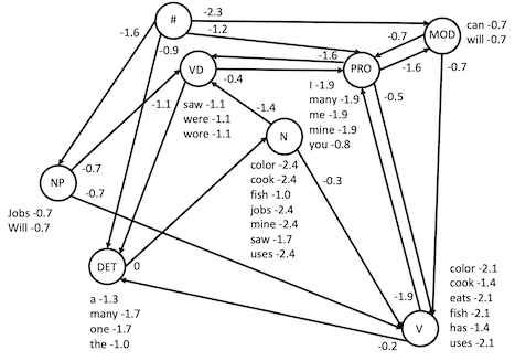
Do you see how the various sentences above follow paths through the HMM? For example, "I fish": transition from start to PRO (score -1.2); observe "I" (score -1.9); transition to V (-0.5); observe "fish" (-2.1). Likewise "Will eats the fish": start to NP (-1.6); "Will" (-0.7); to V (-0.7); "eats" (-2.1); to DET (-0.2); "the" (-1.0); to N (0); "fish" -1.0.
Of course, we as people know the parts of speech these words play in these sentences, and can figure out which paths are being followed. The goal of tagging is to have an algorithm determine what is the best path through the POS states to have produced the observed words. Given the many different out edges, even in this relatively simple case, along with the ambiguity in how words can be used, a proper implementation of the Viterbi algorithm is required to efficiently find the best path.
It could be fun to take a random walk on the HMM to generate new sentences, mad libs style.
POS Viterbi
Let's assume for now we have the model pictured above, and want to find the best path for a given sentence. We'll soon turn to how to obtain the transition and observation probabilities. The Viterbi algorithm starts at the # (start) state, with a score of 0, before any observation. Then to handle observation i, it propagates from each reached state at observation i-1, following each transition. The score for the next state as of observation i is the sum of the score at the current state as of i-1, plus the transition score from current to next, plus the score of observation i in the next. As with Dijkstra, that score may or may not be better than the score we already have for that state and observation — maybe we could get there from a different state with a better overall score. So we'll propagate forward from each current state to each next and check whether or not we've found something better (as with Dijkstra relax).
Let's start by considering "will eats the fish". Starting from #, we can transition to NP, DET, PRO, or MOD. There's an observation score for "will" only in NP and MOD, so what score do we give for observing it in the others? Maybe we don't want to completely rule out something that we've never seen (e.g., "will" can be a noun too, just not in the sentences used to build this model). So let's just give it a low log probability, call it the "unseen" score. It should be a negative number, perhaps worse than the observed ones but not totally out of the realm. For this example, I'll make it -10. So as of word 0, we could be at:
- DET: 0 (current) -0.9 (transition) -10 (unseen observation) = -10.9
- MOD: 0 (current) -2.3 (transition) -0.7 (observation) = -3.0
- NP: 0 (current) -1.6 (transition) -0.7 (observation) = -2.3
- PRO: 0 (current) -1.2 (transition) -10 (unseen observation) = -11.2
The next word, word 1, is "eats". We consider each transition from each of the current states, adding the current score plus the transition plus the observation. From DET we can go to:
- N: -10.9 (current) +0 (transition) -10 (unseen observation) = -20.9
And from MOD to:
- PRO: -3.0 (current) -0.7 (transition) -10 (unseen observation) = -13.7
- V: -3.0 (current) -0.7 (transition) -2.1 (observation) = -5.8
From NP to:
- V: -2.3 (current) -0.7 (transition) -2.1 (observation) = -5.1
- VD: -2.3 (current) -0.7 (transition) -10 (unseen observation) = -13.0
From PRO to:
- MOD: -11.2 (current) -1.6 (transition) -10 (unseen observation) = -22.8
- V: -11.2 (current) -0.5 (transition) -2.1 (observation) = -13.8
- VD: -11.2 (current) -1.6 (transition) -10 (unseen observation) = -22.8
Note that there are several different ways to get to V for word 1 — from MOD (score -5.8), from NP (score -5.1), or from PRO (score -13.8). We keep just the best score -5.1, along with a backpointer saying that V for word 1 comes from NP for word 0. Similarly VD for word 1 could have come from NP or PRO, and we keep its best score of -13.0 with a backpointer to NP for word 0.
To continue on, I think it's easier to keep track of these things in a table, like the following, where I use strikethrough to indicate scores and backpointers that aren't the best way to get to the next state for the observation. (Apologies if I added anything incorrectly when I manually built this table — that's why we have computers; let me know and I'll fix it.)
| # | observation | next state | curr state | scores: curr + transit + obs | next score |
|---|---|---|---|---|---|
| start | n/a | # | 0 | n/a | 0 |
| 0 | will | DET | # | 0 -0.9 -10 | -10.9 |
| MOD | # | 0 -2.3 -0.7 | -3.0 | ||
| NP | # | 0 -1.6 -0.7 | -2.3 | ||
| PRO | # | 0 -1.2 -10 | -11.2 | ||
| 1 | eats | N | DET | -10.9 +0 -10 | -20.9 |
| PRO | MOD | -3.0 -0.7 -10.0 | -13.7 | ||
| V | -3.0 -0.7 -2.1 | ||||
| -11.2 -0.5 -2.1 | |||||
| NP | -2.3 -0.7 -2.1 | -5.1 | |||
| VD | NP | -2.3 -0.7 -10 | -13.0 | ||
| -11.2 -1.6 -10 | |||||
| MOD | PRO | -11.2 -1.6 -10 | -22.8 | ||
| 2 | the | DET | V | -5.1 -0.2 -1.0 | -6.3 |
| -13.0 -1.1 -1.0 | |||||
| MOD | PRO | -13.7 -1.6 -10 | -25.3 | ||
| PRO | V | -5.1 -1.9 -10 | -17.0 | ||
| -13.0 -0.4 -10 | |||||
| -22.8 -0.7 -10 | |||||
| V | -20.9 -0.3 -10 | ||||
| PRO | -13.7 -0.5 -10 | -24.2 | |||
| -22.8 -0.7 -10 | |||||
| VD | -20.9 -1.4 -10 | ||||
| PRO | -13.7 -1.6 -10 | -25.3 | |||
| 3 | fish | DET | V | -24.2 -0.2 -10 | -34.4 |
| -25.3 -1.1 -10 | |||||
| MOD | PRO | -17 -1.6 -10 | -28.6 | ||
| N | DET | -6.3 +0 -1.0 | -7.3 | ||
| PRO | -25.3 -0.7 -10 | ||||
| -24.2 -1.9 -10 | |||||
| VD | -25.3 -0.4 -10 | -35.7 | |||
| V | -25.3 -0.7 -2.1 | ||||
| PRO | -17.0 -0.5 -2.1 | -19.6 | |||
| VD | PRO | -17.0 -1.6 -10 | -28.6 |
Important: We are not deciding for each word which tag is best. We are deciding for each POS tag that we reach for that word what its best score and preceding state are. This will ultimately yield the best path through the graph to generate the entire sentence, disambiguating the parts of speech of the various observed words along the way.
After working through the sentence, we look at the possible states for the last observation, word 3, to see where we could end up with the best possible score. Here it's N, at -7.3. So we know the tag for "fish" is N. We then backtrace to where this state came from: DET. So now we know the tag for "the" is DET. Backtracing again goes to V, for "eats". Then back to NP, for "will". Then #, so we're done. The most likely tags for "Will eats the fish" are: NP V DET N
POS Training
Let's consider training the pictured model from the example sentences and corresponding tags. Basically, we just go through each sentence and count up, for each tag, how many times each word was observed with that tag, and how many times each other tag followed it. So we essentially want to collect tables (or really maps) like these:
| Transitions | Observations | ||||||||||||||||||||||||||||||||||||||||||||||||||||||||||||||||||||||||||||||||||||||||||||||||||||||||||||||||||||||||||||||||||||||||||||||||||||||||||||||||||||||||||||||||
|
| ||||||||||||||||||||||||||||||||||||||||||||||||||||||||||||||||||||||||||||||||||||||||||||||||||||||||||||||||||||||||||||||||||||||||||||||||||||||||||||||||||||||||||||||||
The first sentence "I/PRO fish/V" puts a 1 in the transition from # to PRO, along with a 1 in that from PRO to V. It also puts a 1 in the observation of "i" in PRO and that of "fish" in V. The next sentence "Will/NP eats/V the/DET fish/N" puts a 1 in transitions # to NP, NP to V, V to DET, and DET to N. It likewise puts 1 in observations "will" in NP, "eats" in V, "the" in DET, and "fish" in N. The third sentence "Will/MOD you/PRO cook/V the/DET fish/N" puts a 1 in transitions # to MOD and MOD to PRO; it increments by 1 the transition PRO to V (already had 1 from the first sentence) along with V to DET and DET to N (both already had 1 from the second sentence). It also puts a 1 for "will" in MOD, "you" in PRO, and "cook" in V, while incrementing by 1 both "the" in DET and "fish" in N (already had 1 from the second sentence). Thus we have:
| Transitions | Observations | ||||||||||||||||||||||||||||||||||||||||||||||||||||||||||||||||||||||||||||||||||||||||||||||||||||||||||||||||||||||||||||||||||||||||||||||||||||||||||||||||||||||||||||||||
|
| ||||||||||||||||||||||||||||||||||||||||||||||||||||||||||||||||||||||||||||||||||||||||||||||||||||||||||||||||||||||||||||||||||||||||||||||||||||||||||||||||||||||||||||||||
Finally, we convert these counts to log probabilities, by dividing each by the total for its row and taking the log. With only limited experience of 3 sentences, this HMM has only seen one type of transition from each state other than the start state, and has only limited vocabulary of one or two words for each state. So the transition probabilities from # to each of MOD, NP, and PRO is log (1/3), while that from DET to N is log (2/2) = 0. Likewise, the observation of each of "cook", "eats", and "fish" in V is log (1/3), while that of "i" and "you" in PRO is log (1/2). But if we trained it on the rest of the example sentences, we'd have a somewhat more interesting set of transition and observation counts, whose conversion yields the numbers I gave on the figure (rounded off).
Testing
To assess how good a model is, we can compute how many tags it gets right and how many it gets wrong on some test sentences. (Even tougher: how many sentences does it get entirely right vs. at least one tag wrong.) It wouldn't be fair to test it on the sentences that we used to train it (though if it did poorly on those, we'd be worried).
Provided in texts.zip are sets of files, one pair with the sentences and a corresponding one with the tags to be used for training, and another pair with the sentences and tags for testing. Each line is a single sentence (or a headline), cleanly separated by whitespace into words/tokens, with punctuation also thus separated out. Note the lines corresponds token-to-tag — the 0th token on a line in the text file has the 0th token in the same line in the tags file, ... the ith token has the i tag, .... (And that also applies to punctuation, corresponding token-to-tag mixed in among the words.)
So use the train sentences and train tags files to generate the HMM. Then apply the HMM to each line in the test sentences file, and compare the results to the corresponding test tags line. Count the numbers of correct vs. incorrect tags.
Implementation Notes
Training- I preserved capitalization in the examples, but lowercasing all the words makes sense.
- While we think of the model as a graph, you need not use the Graph class, and you might in fact find it easier just to keep your own Maps of transition and observation probabilities as we did with finite automata. Think first about what the mapping structure should be (from what type to what type). Recall that you can nest maps (the value for one key is itself a map). The finite automata code might be inspiring, but remember the differences (e.g., HMM observations are on states rather than edges; everything has a log-probability associated with it).
- Make a pass through the training data just to count the number of times you see each transition and observation. Then go over all the states, normalizing each state's counts to probabilities (divide by the total for the state). Remember to convert to log probabilities so you can sum the scores. (FWIW, the sample solution uses natural log, not log10.)
- While the table shows all the scores, we really need only to keep the current ones and the next ones, as shown in the pseudocode in the lecture notes. So that might simplify the representation you use.
- Warning: it would be highly inefficient to keep a list of all next states, as there is redundancy in how to get to each, i.e., the same state could be added multiple times (as we see with V from MOD, PRO, and NP even in this simple example). And this only gets exponentially worse as you proceed through Viterbi.
- The backtrace, on the other hand, needs to go all the way back: for observation i, for each state, what was the previous state at observation i-1 that produced the best score upon transition and observation. Note that if we index the observations by numbers, as suggested here, the representation is essentially a list of maps.
- After handling the special case of the start state, start for real with observation 0 and work forward. Either consider all possible states and look back at where they could have come from, or consider all states from which to come and look forward to where they could go. In either case, be sure to find the max score (and keep track of which state gave it).
- Use a constant variable for the observation of an unobserved word, and play with its value.
- The backtrace starts from the state with the best score for the last observation and works back to the start state.
Exercises
For this assignment, you may work either alone, or with one other partner. Same discussion as always about partners.
- Write a method to perform Viterbi decoding to find the best sequence of tags for a line (sequence of words).
- Test the method on simple hard-coded graphs and input strings (e.g., from programming drill, along with others you make up). In your report, discuss the tests and how they convinced you of your code's correctness.
- Write a method to train a model (observation and transition probabilities) on corresponding lines (sentence and tags) from a pair of training files.
- Write a console-based test method to give the tags from an input line.
- Write a file-based test method to evaluate the performance on a pair of test files (corresponding lines with sentences and tags).
- Train and test with the two example cases provided in texts.zip: "example" are the sentences and tags above, "simple" is just some made up sentences and tags, and "brown" is the full corpus of sentences and tags. The sample solution got 32 tags right and 5 wrong for simple, and 35109 right vs. 1285 wrong for brown, with an unseen-word penalty of -100. (Note: these are using natural log; if you use log10 there might be some differences.) In a short report, provide some example new sentences that are tagged as expected and some that aren't, discussing why. Also discuss your overall testing performance, and how it depends on the unseen-word penalty (and any other parameters you use).
Some ideas for extra credit.
- Move from bigrams to trigrams (i.e., a tag depends on the previous two tags). Compare performance.
- Be more careful with things that haven't been observed; this is even more necessary with trigrams. One approach is "interpolation": take a weighted sum of the unigram, bigram, and trigram probabilities, so that the less-informative but more-common lower-order terms can still contribute.
- Perform cross-validation. Randomly split the data into different partitions (say 5 different groups, or "folds"). Set aside part 0, train on parts 1-4, and then test on part 0. Then set aside part 1, train on parts 0 & 2-4, and test on 1. Etc. So each part is used as a test set, with the other parts used in training, to construct the model. Note that the Brown corpus is organized by genre (news, fiction, etc.), so deal out the rows among the partitions instead of assigning the first n/5 to one group, the second n/5 to the next, etc.
- Use your model generatively. This can be done randomly (essentially following a path through the HMM, making choices according to the probabilities), or predictively (identify what the best next word would be to continue a sentence).
- Use a different corpus; e.g., from phonemes to morphemes, or from one language to another.
Submission Instructions
Turn in a single zipfile containing all your code and your short report (testing on hard-coded graphs, training/testing on provided datasets).
Acknowledgment
Thanks to Professor Chris Bailey-Kellogg for a rewrite of this problem that greatly clarifies the details around scoring. Also thanks to Sravana Reddy for consulting in the development of the problem set, providing helpful guidance and discussion as well as the processed dataset.
Grading rubric
Total of 100 points
Correctness (70 points)
| 5 | Loading data, splitting into lower-case words |
|---|---|
| 15 | Training: counting transitions and observations |
| 5 | Training: log probabilities |
| 15 | Viterbi: computing scores and maintaining back pointers |
| 5 | Viterbi: start; best end |
| 10 | Viterbi: backtrace |
| 7 | Console-driven testing |
| 8 | File-driven testing |
Structure (10 points)
| 4 | Good decomposition into objects and methods |
|---|---|
| 3 | Proper use of instance and local variables |
| 3 | Proper use of parameters |
Style (10 points)
| 3 | Comments for classes and methods |
|---|---|
| 4 | Good names for methods, variables, parameters |
| 3 | Layout (blank lines, indentation, no line wraps, etc.) |
Testing (10 points)
| 5 | Example sentences and discussion |
|---|---|
| 5 | Testing performance and discussion |