Shortest paths
BFS works well to find paths with the minimum number of edges, as in the Kevin Bacon Game. However, many times we will have graphs where the edges have weights, e.g., in a map (of the cartographic kind) where the edges are roads connecting cities, and we want shortest-total-distance routes. Similarly the weight on each road could represent how long it would take to go that way, and we want fastest routes. And of course, the graph could represent other connections, e.g., in a network.
Code for today: a bunch of classes in mazeSearch.zip with data in mazes.zip.
Shortest-path simulation
There are a number of different path-finding problems, but we will discuss what is called the "single-source shortest path" problem — all shortest paths from a single node (just like BFS giving fewest-edge paths from a single node). If there are no negative edge weights, then this can be solved by a generalization of BFS called Dijkstra's Algorithm, named after its inventor.
Dijkstra's algorithm finds a shortest path from a source vertex s to all other vertices. We'll compute, for each vertex v, the weight of a shortest path from the source to v, which we'll denote by v.dist. Now, this notation presumes that we have an instance variable dist for each vertex. We don't have to store shortest-path weights as instance variables. For example, we can use a map instead, mapping each vertex to its shortest-path weight. But for the purpose of understanding the algorithm, we'll use v.dist. We will also keep track of the back-pointer on each shortest path. Standard nomenclature for a back-pointer on a shortest path is a predecessor, and so we'll denote the predecessor of vertex v on a shortest path from the source by v.pred. As with the back-pointers in BFS, the predecessors in shortest paths form a directed tree, with edges pointing on paths toward the source.
I like to think of Dijkstra's algorithm as a simulation of sending out runners over the graph, starting at the source vertex. Ideally, the simulation works as follows, though we'll see that Dijkstra's algorithm works slightly differently. It starts by sending out runners from the source vertex to all adjacent vertices. The first time a runner arrives at any vertex, runners immediately leave that vertex, headed to all of its adjacent vertices. Look at part (a) of this figure:
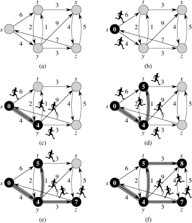
It shows a directed graph with source vertex s and weights next to the edges. Think of the weight of an edge as the number of minutes it would take a runner to traverse the edge.
Part (b) illustrates the start of the simulation, at time 0. At that time, shown inside vertex s, runners leave s and head toward its two adjacent vertices, t and y. The blackened vertex s indicates that we have determined the value of s.dist (which is 0).
Four minutes later, at time 4, the runner to vertex y arrives, shown in part (c). Because this runner is the first to arrive at y, we know that y.dist = 4, and so y is blackened in the figure. The shaded edge (s, y) indicates that the first runner to arrive at vertex y came from vertex s, so that y.pred = s. At time 4, the runner from vertex s to vertex t is still in transit. Runners leave vertex y at time 4, headed toward vertices t, x, and z.
The next event, displayed in part (d), occurs one minute later, at time 5, when the runner from vertex y arrives at vertex t. The runner from s to t has yet to arrive. Because the first runner to arrive at vertex t arrived from vertex y at time 5, we set t.dist to 5 and t.pred to y (indicated by the shaded edge (y, t)). Runners leave vertex t, headed toward vertices x and y at this time.
The runner from vertex s finally arrives at vertex t at time 6, but the runner from vertex y had already arrived there a minute earlier, and so the effort of the runner from s to t went for naught.
At time 7, depicted in part (e), two runners arrive at their destinations. The runner from vertex t to vertex y arrives, but the runner from s to y had already arrived at time 4, and so the simulation forgets about the runner from t to y. At the same time, the runner from y arrives at vertex z. We set z.dist to 7 and z.pred to y, and runners leave vertex z, headed toward vertices s and x.
The next event occurs at time 8, as shown in part (f), when the runner from vertex t arrives at vertex x. We set x.dist to 8 and x.pred to t, and a runner leaves vertex x, heading to vertex z.
At this point, every vertex has had a runner arrive, and the simulation can stop. All runners still in transit will arrive at their destination vertices after some other runner had already arrived. Once every vertex has had a runner arrive, the distvalue for each vertex equals the weight of the shortest path from vertex s and the pred value for each vertex is the predecessor on a shortest path from s.
Dijkstra's algorithm
That was how the simulation proceeds ideally. It relied on the time for a runner to traverse an edge equaling the weight of the edge. Dijkstra's algorithm works slightly differently. It treats all edges the same, so that when it considers the edges leaving a vertex, it processes the adjacent vertices together, and in no particular order. For example, when Dijkstra's algorithm processes the edges leaving vertex s, it declares that y.dist = 4, t.dist = 6, and y.pred and t.pred are both s — so far. When Dijkstra's algorithm later considers the edge (y, t), it decreases the weight of the shortest path to vertex t that it has found so far, so that t.dist goes from 6 to 5 and t.pred switches from s to y.
Dijkstra's algorithm maintains a min-priority queue of vertices, with their dist values as the keys. It repeatedly extracts from the min-priority queue the vertex u with the minimum dist value of all those in the queue, and then it examines all edges leaving u. If v is adjacent to u and taking the edge (u, v) can decrease v's dist value, then we put edge (u, v) into the shortest-path tree (for now, at least), and adjust v.dist and v.pred. Let's denote the weight of edge (u, v) by w(u,v). We can encapsulate what we do for each edge in a relaxation step, with the following pseudocode:
void relax(u, v) {
  if (u.dist + w(u,v) < v.dist) {
    v.dist = u.dist + w(u,v);
    v.pred = u;
  }
}
Whenever a vertex's dist value decreases, the min-priority queue must be adjusted accordingly.
Here is pseudocode for Dijkstra's algorithm, assuming that the source vertex is s:
void dijkstra(s) {
  queue = new PriorityQueue<Vertex>();
  for (each vertex v) {
    v.dist = infinity;  // can use Integer.MAX_VALUE or Double.POSITIVE_INFINITY
    queue.enqueue(v);
    v.pred = null;
  }
  s.dist = 0;

  while (!queue.isEmpty()) {
    u = queue.extractMin();
    for (each vertex v adjacent to u)
      relax(u, v);
  }
}
In the following figure, each part shows the dist value (appearing within each vertex), the pred value (indicated by shaded edges), and the vertices in the min-priority queue (the vertices that are shaded, not blackened) just before each iteration of the while-loop:

The vertex that is newly blackened in each part of the figure is the vertex chosen as vertex u in in each iteration of the while-loop. In the simulation with runners, once a vertex receives dist and pred values, they cannot change, but here a vertex could receive dist and pred values in one iteration of the while-loop, and a later iteration of the while-loop for some other vertex u could change these values. For example, after edge (y, x) is relaxed in part (c) of the figure, the value of x.dist decreases from ∞ to 13, and x.pred becomes y. The next iteration of the while-loop in (part (d)) relaxes edge (t, x), and x.dist decreases further, to 8, and x.pred becomes t. In the next iteration (part (e)), edge (z, x) is relaxed, but this time x.dist does not change, because its value, 8, is less than z.dist + w(z,x), which equals 12.
When implementing Dijkstra's algorithm, we must take care that the min-priority queue is updated whenever a dist value decreases. For example, the implementation in the textbook uses a HeapAdaptablePriorityQueue, which has a method replaceKey. This method updates the min-priority queue's internal state to reflect the change in a vertex's key. The textbook also relies on a map from Vertex objects to Entry objects, which locate the vertex in the min-priority queue. It's a bit complicated.
Let's consider the run-time complexity of the algorithm. We add each vertex to the PQ once, remove it as the min once, and relax each edge (and perhaps reduce a key) once. So this is O(n*(insert time + extractMin time) + m*(reduceKey time)). So how long this is depends on the time to insert and extractMin in a priority queue and on the time to reduce a key. The natural way to do this is to use a heap-based PQ as the book does. Then each operation takes O(log n), for a total of O(n log n + m log n).
An alternate approach (that seems pretty stupid) is to keep an unordered list for the PQ. Then insert takes O(1), extractMin takes Θ(n), and reduceKey takes O(1) (if you have position-aware vertices so can find where a vertex is in the list in O(1) time). So this takes O(n2 + m) time. This is clearly worse. Except it isn't. If the graph has lots of edges and m = Θ(n2) this is Θ(n2). The "clever" approach is Θ(n2 log n)! This was an embarrassment for decades. Eventually a type of priority queue called a Fibonacci Heap was invented, which has O(1) amortized time for reduceKey. So the run time is O(n log n + m), which is O(n2).
A* search
If we are trying to go from Hanover to Boston does it make sense to calculate distances to Montpelier and Burlington?. Of course not. We are going in the "wrong direction." But Dijkstra's algorithm would calculate these distances, because they are closer to Hanover than Boston. How could Dijkstra's algorithm know that looking at Montpelier and Burlington is a waste of time?
If we are looking for the shortest path to a known goal we can use a generalization of Dijkstra's algorithm called A* search to find the shortest path without taking as much time as normal Dijkstra's. The idea is to use an estimate the distance remaining, and to add it to the distance traveled so far to get the key for the city in the PQ. For this case the normal Euclidean distance between Montpelier and Boston would be something like 130 miles. (Figure this Euclidean distance from GPS coordinates of longitude and latitude.) Adding this to the 45 miles from Hanover to Monpelier would give 175 miles. Therefore Boston (whose distance will be 120 miles or so) would come out of the PQ before Montpelier.
Just as in Dijkstra's algorithm, in A* we have a PQ and a "closed set" of vertices where we know the best path, so if we discover them again while searching we don't need to deal with them. The second group is the "open set" corresponding to vertices in the PQ. Just as in Dijkstra's when we extractMin from the PQ we move the corresponding vertex to the cloud (closed set) and remove it from the PQ and the open set. We then find incident edges and relax them (update a adjacent vertex's current distance if we have found a shorter path). But the key in the PQ is always distance so far plus the estimate of the remaining distance.For this to find the shortest path we need two things. First, the estimate of distance remaining must be admissible. This means that we always underestimate the true remaining distance or get it exactly. Because of the triangle inequality the Euclidean distance is an underestimate of the true travel distance. In fact, the ultimate underestimate of the remaining distance is 0. This leads to normal Dijkstra, because then we take the shortest distance traveled next.
The second requirement is that the cost estimate is monotone. That means that if we extend the path (thus increasing the distance travelled so far), the total estimate is never less that the estimate before we extended the path. This is the generalization of "no negative edges." Our Euclidean distance plus distance so far estimate satisfies this, because if moving to an adjacent vertex increases the distance so far by d it cannot reduce the Euclidean distance by more than d. (It would reduce by exactly d if you were moving directly toward the goal.) Thus the sum will not go down. Using just Euclidean distance (without distance so far) would fail to be monotone, so would not be not guaranteed to give shortest paths.
Implicit graphs
We often deal with problems where the graph is implicit. Consider a maze. There is an underlying graph — the squares in the maze are the vertices and the edges connect adjacent squares. However, to convert the maze to a graph is more effort than to find the shortest path, because we end up converting parts of the maze that we would never visit. What is worse is a puzzle like the 15-puzzle (15 numbered tiles and a blank in a 4x4 frame, with the tiles able to slide into the blank's position) or Rubic's Cube. Here the size of the implicit graph is potentially enormous. Therefore we create vertex objects as we need them and find adjacencies on the fly. (For the 15-puzzle two configurations are adjacent if they differ by sliding one tile into the blank position and for Rubic's cube two configurations are adjacent if they differ by a twist.)
Suppose we want to find paths in a maze. Here's a whole GUI application for stepping through various searches: mazeSearch.zip; and here are some example mazes: mazes.zip (the application assumes they're saved in the "data" folder parallel to the "src" folder containing the code). Fire it up from "MazeSolver.java".
Here's an example of the type of maze:
**********
*S* **   *
*      * *
* **** * *
*   **** *
*** *T   *
**********
Note that *s represent walls, S and T represent the start and goal, respectively, and empty spaces delineate the actual paths through the maze.
DFS can lead to very long paths. (Example: maze5.) BFS will guarantee finding the shortest path, but can be very slow. We can improve on DFS by using a heuristic, e.g. the L1 (Manhattan) distance from where we are to the target square. (This means adding the x difference to the y difference between the two squares.) If we use a PQ based on this distance we will tend to "zoom in" on the target. However, this will not guarantee a shortest path. (Again demo the maze program.) Can we do better?
int dist = Math.abs(row-targetRow) + Math.abs(col-targetCol);Using A* search we can find the shortest path without taking as much time as BFS. The idea is to add a heuristic like the L1 distance to estimate the distance remaining. For our maze the L1 distance is an admissible estimate — we move either horizontally or vertically in each step, so the number of steps needed is at least the L1 distance. Note we could also have used the Euclidean distance. That would be a bigger underestimate, because the Euclidean distance will usually be smaller than the L1 distance and will never be larger. Demo on maze5, showing that the square where the paths meet will be discovered from the right first, but will be eventually included in the path from the left. Note that using a remaining distance estimate of 0 gives BFS on the implicit maze graph, because the shortest path is always expanded next.
Now let's look at the code. It uses a "sequencing" mechanism to keep track of what to visit next. The Sequencer basically generalizes the various ways we've seen to establish order — stack, queue, priority queue. Elements are added to the Sequencer, and on request it returns the next one by whatever order it maintains. Its elements are SequenceItem instances. Here, they're specialized to rows and columns in the maze, but we could make them generic by requiring that they implement an appropriate interface. Note that we define an equals method to declare two items equal if their rows and columns are equal, and we override hashCode so that the hashCodes of equal items are equal.
The stepMaze method of Maze does the real work of the application. It calls the sequencer to get the next maze square to be processed. If the square to be processed is the target it traces back the path, marking each square as on the final path. If not, and the square was not explored, it tries to add each of its four potential neighbors to the sequencer (if they exist and are either empty or the target) and marks the current square as explored. This will prevent it from being explored again later.
public void stepMaze() {
  if (!isDone && theMaze != null)
    if (!seq.hasNext())
      isDone = true;
    else {
      SequenceItem current = seq.next();
      int row = current.getRow();
      int col = current.getCol();
      if (theMaze[row][col] == TARGET) {
        isDone = true;
        tracePath(current.getPrevious());
      }
      else if (theMaze[row][col] == EMPTY || theMaze[row][col] == START) {
        addIfValid(row-1, col, current);
        addIfValid(row+1, col, current);
        addIfValid(row, col-1, current);
        addIfValid(row, col+1, current);
        if (theMaze[row][col] == EMPTY) // Don't change START
          theMaze[row][col] = EXPLORED;
      }
    }
}
The actual code for solving the maze would have been simpler if we were not creating an interactive GUI. The GUI requires spreading the solution out, separating out the code for taking a step and making it act on the current "state" of the maze. This step code would normally be part of a loop. But here the loop is provided by the GUI, either via the Step button or repeated calls from the Timer after clicking Solve. The GUI implementation has more lower level Java stuff than the GUIs we've looked at so far, so ignore the details for now.
We have a bunch of different ways to search, via different subclasses of Sequencer. StackSequencer and QueueSequencer use a stack and queue, respectively, to add and get the next item. DistSequencer uses a priority queue, where the priority is the L1 distance to the target. This distance gets saved in the key field in the PQSequenceItem and is used when comparing items in the priority queue. Finally AStarSequencer keeps track of the open set via a map from SequenceItems to entries in the PQ, so that when we find a shorter distance we can find and update the appropriate PQ entry. It uses an AdaptablePriorityQueue from the book to allow the value of an entry's key to be changed when relaxation finds a better path. The AStarSequenceItem has an instance variable to hold the path length and a method get it, because that is part of the estimate.
Note: if you want to run this yourself, since it uses code from the book, you'll need to download the jar file from the book website and add it to your project (as with JavaCV, way back at the start of the term — menu Project | Properties | Java Build Path | Libraries | Add External JARS....).