Pattern recognition
We saw last time how to match precisely specified patterns in strings. But what if there's some uncertainty / slop in what's allowed to match? Handling uncertainty is necessary, e.g., in speech recognition and similar problems, where the input is noisy and the rules for matching (converting sounds to pieces of words, pieces of words to words, words to sentences, etc.) are far from perfect. Such problems are called "pattern recognition" problems — related to pattern matching, but allowing for uncertainty/noise and trying to determine the best possible explanation for the data. This is our CS 10 taste test of machine learning. One powerful approach useful in pattern recognition is called a hidden Markov model (HMM), which allows the recognition of sequences (words, music, biological sequences, smartphone sensor patterns). Often we use these sequences to infer something that we cannot directly measure. For example, we cannot directly measure if someone is depressed, but we may be able to infer it using sensor data such as: GPS data to know if the person leaves home frequently or tends to stay inside, microphone data to know if the person speaks with other people often or if they tend to keep quiet and avoid conversations with others, etc.
From FA to HMM
As with finite automata, a hidden Markov model is driven by transitions from state to state. Which transitions are allowed depends only on the current state, not the history of how we got there. (That's the "Markov" property in the name of the model.) Different from FAs, in HMMs the outputs (matched characters or whatever) are handled at the states instead of on the transitions. So in our road trip analogy, instead of giving a token to travel down a road, we give a token upon arriving in a city. The other major difference is that we put weights on everything. Just as Dijkstra generalized BFS to compute shortest paths by an arbitrary (non-negative) weight instead of just the number of edges, HMMs allow finding "best" paths (by weight) matching the input. In contrast, for DFAs there was only one path, and NFAs found all matching paths without providing any guidance on one vs. another.
Back to our road trip analogy from FA. The path through an HMM is characterized by a sequence of observations (one per vertex), serving much the same role as tokens in an FA (one per edge). So in our road trip, the observations would be, say, an activity for each day (in a particular city that day). As with tokens, these are in order — first day hiking, second day eating great food, third day at the beach, fourth day in a museum, etc. An HMM road trip has a weight for everything. We'll make the weights represent "desirability", so that larger is better, say on a scale 1-10 (with 0 meaning not possible). The weight for a road represents how desirable it is to drive it (time / distance / money / scenery), while the weight for an activity at a city represents how well that city supports that activity. Some cities are really good for art museums, some not so good. Some we like to stay multiple days in (self edges), others not. And remember, we have a planned itinerary of activities. So then even if there's a desirable connection from the city we're in now to another city, we might not go there next if it rates poorly for what we want to do the next day. The overall path will take desirable steps in an order that puts us in desirable cities according to our activity plan, maximizing the overall desirability of activities and connections.
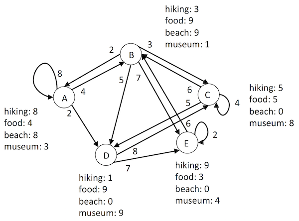
While we've been thinking about this from a road trip planning perspective, we could imagine it from a road trip "decoding" perspective. You show your friend a series of photos — first day on a mountain, second day with a plate of yummy food, third day surfing, fourth day in front of a Monet, etc. Then you ask them to infer which city you were in each day. They have a sense of how good each city is for each activity, and how much you might like taking a particular connection (or staying in a city multiple days). Thus they can make a reasonable guess of your path. That's where the "hidden" part in HMM comes from. Your friend knows what you've done (in order), but not where you've been to do it, and is trying to infer your path (initially hidden to them).
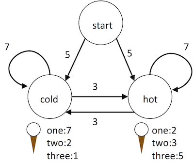
For another example, consider the case of the future archaeologist trying to infer the weather from a diary keeping track of the number of ice cream cones someone ate each day [due to Jason Eisner]. The archaeologist doesn't know the weather each day — it's the hidden state, either cold or hot. The only observations are the number of cones eaten, as recorded in the diary. Transitions indicate whether the actual weather stays the same (likely — higher weight edge) or switches (less likely — lower weight), from day to day. The number of cones eaten for the day depends on whether it was hot (higher weights for larger numbers of cones) or cold (higher weights for smaller numbers of cones). And somehow the whole process gets started, so we have a "start" state with equally likely transitions to go to a hot day or a cold day.
Real examples abound, in language understanding, sensor processing, music analysis, evolutionary modeling, etc. You'll do one of these, trying to infer the hidden part of speech for each observed word in a sentence; ambiguity arises because some words can be different parts of speech in different contexts (e.g. "present": I could present you with a present). At a lower level, we could try to infer the actual word from composition of "parts" (phonemes, like long A vs. short A), or in the other direction try to infer how to say a word from its spelling (should that be a long or short sound). And at a higher level we could try to infer the corresponding foreign language words for a given sentence.
Decoding: Viterbi algorithm
Let's look at an algorithm to figure out the best (or most likely) path taken through a graph to produce an observed sequence. In the road trip, that was your friend trying to figure out where you were each day based on your photos. In the ice cream meteorology example, suppose we observe this sequence in the journal: 2 cones, then 3 cones, then 2 cones, then 1 cone, ... What was the weather pattern? It could have been hot, then hot, then hot, then cold; or maybe it was cold, then hot, then hot, then cold; or maybe hot all four days; etc. We want to determine the best possible path, based on scores we give to eating numbers of cones on hot days vs. on cold days, and on changing from hot to cold and vice versa. Since there are an exponential number of possibilities, we clearly can't just enumerate all of them and score, so we need a clever algorithm.
The algorithm for decoding (determining the best path) was developed by Viterbi back in 1967 (though not specific to HMMs), and has really driven the utility of HMMs, as it provides an efficient way to do that without considering all the exponential combinations. One way to approach it feels an awful lot like the way we considered paths through an NFA (which in turn is much like the way we considered paths through a Kevin Bacon graph, though keeping a whole pond ripple together rather than using a queue). We repeatedly expand outward from the start state, keeping the set of the next states we could reach.
So we start at the start state, before any observations. We take one step at a time, advancing from each state we could be in now, to each other one that could follow it. In so doing, we produce the next observation at each such next state. Thus we expand from the start state before any observations, follow all its transitions to get to the states where the first observation could have be made, follow all their transitions to get to where the second one could have been made, etc. Now we also have the scores to take care of. So when moving from one state to the next, we add the score of the edge from the current to the next, and the score of the next observation in the next state. E.g., if we step from "hot" to "cold" corresponding to an observed journal entry with 3 ice cream cones, then we add the score of the hot → cold edge and the score of 3 cones on a cold day. There might be multiple ways to arrive at a state. With NFA, we used a Set so they all collapsed down. Here, we want the best possible one, in terms of "desirability". So each time we transition to a state for an observation, we take the max of the current best score for that vs. the new one.
In pseudocode:
currStates = { start }
currScores = map { start=0 }
for i from 0 to # observations - 1
  nextStates = {}
  nextScores = empty map
  for each currState in currStates
    for each transition currState -> nextState
      add nextState to nextStates
      nextScore = currScores[currState] +                       // path to here
                  transitionScore(currState -> nextState) +     // take a step to there
                  observationScore(observations[i] in nextState) // make the observation there
      if nextState isn't in nextScores or nextScore > nextScores[nextState]
        set nextScores[nextState] to nextScore
        remember that pred of nextState @ i is curr
  currStates = nextStates
  currScores = nextScores
For the ice cream example, with the observation sequence (two cones, three, two, one), trying to figure out the weather:
| # | observation | nextState | currState | currScore + transitScore + obsScore | nextScore |
|---|---|---|---|---|---|
| start | n/a | start | n/a | 0 | 0 |
| 0 | two cones | cold | start | 0 + 5 + 2 | 7 |
| hot | start | 0 + 5 + 3 | 8 | ||
| 1 | three cones | cold | cold | 7 + 7 + 1 | 15 |
| hot | 8 + 3 + 1 | ||||
| hot | cold | 7 + 3 + 5 | |||
| hot | 8 + 7 + 5 | 20 | |||
| 2 | two cones | cold | cold | 15 + 7 + 2 | |
| hot | 20 + 3 + 2 | 25 | |||
| hot | cold | 15 + 3 + 3 | |||
| hot | 20 + 7 + 3 | 30 | |||
| 3 | one cone | cold | cold | 25 + 7 + 7 | |
| hot | 30 + 3 + 7 | 40 | |||
| hot | cold | 25 + 3 + 2 | |||
| hot | 30 + 7 + 2 | 39 |
The table is organized around the next observation and the state in which that observation could have been made (nextState). For each such pair, there is a row for each state that could be currState and take a step to nextState. The algorithm fills in the table by looping over the observation # (proceeding through the observations), the current state (where could we be right now), and the possible next states (where could we go for that observation). It adds the current state's score to the score for the transition to the next state and the score for the observation in the next state, and plugs that into the row for the observation in that next state. Thus for observation 0, start as the current state, and cold as the next state, we compute 0 (current score) + 5 (start to cold) + 2 (two cones in cold) and plug that into (0, cold). Then advancing to hot as the next state, we compute 0 (current) + 5 (start to hot) + 3 (two cones in hot) and plug in at (0, hot). Likewise for observation 1, cold as current, and cold as next, we compute 7 (current score) + 7 (cold to cold) + 1 (three cones in cold) and plug in at (1, cold). The table shows both possible currStates, crossing out the smaller score; the larger one is used to propagate further.
Once we've accounted for all the observations, we end up in any number of possible states. (In some HMMs, we only care about a stop state, just like with NFAs, but we won't do that here.) The scores there then indicate the best total score over the possible histories. In the ice cream example, it looks like the best history ended up on a cold day (40 for cold > 39 for hot).
But this just gives us the score. How do we determine the underlying path through the states? Fortunately, we remembered how we got to each state for each observation. So now we just start at the best final state and work backward. The backtracing is much like in BFS, except that it's not just node to previous node, but node at observation to previous node at previous observation. For ice cream, we go from cold at #3; back to its predecessor, hot at #2; back its predecessor, hot at #1; back to its predecessor, hot at #0; back to start.
What if the next day was a three-cone day?
| # | observation | nextState | currState | currScore + transitScore + obsScore | nextScore |
|---|---|---|---|---|---|
| 4 | three cones | cold | cold | 40 + 7 + 1 | 48 |
| hot | 39 + 3 + 1 | ||||
| hot | cold | 40 + 3 + 5 | |||
| hot | 39 + 7 + 5 | 51 |
That changes our inference of history! We ended on a hot day, which came from a hot day (#3), a hot day (#2), a hot day (#1), a hot day (#1). Note that the path now goes through a hot day on #3 instead of a cold day — we find the one globally consistent with them, also accounting for the transitions.
Training
So how do we get the scores for an HMM anyway? In many situations, we have annotated training data. In the road trip example, we could collect ratings from lots of tourists, indicating how much they enjoyed a particular activity in a particular city. Then average those out. While actual road "desirability" might be hard, we could certainly get relative road popularity. In the ice cream example, perhaps the person keeping the journal did annotate the actual weather for a few days, along with the number of ice cream cones. So we can get a sense for the relationship between weather and number of ice cream cones for those days, as well as a sense for the general weather trends (how often it stays hot when it is already, etc.). This lets us then make predictions for the rest of the journal.
Suppose in particular that we had the following journal entries:
- Hot day today! I chowed down three whole cones.
- Hot again. But I only ate two cones; need to run to the store and get more ice cream.
- Cold today. Still, the ice cream was calling me, and I ate one cone.
- Cold again. Kind of depressed, so ate a couple cones despite the weather.
- Still cold. Only in the mood for one cone.
- Nice hot day. Yay! Was able to eat a cone each for breakfast, lunch, and dinner.
- Hot but was out all day and only had enough cash on me for one ice cream.
- Brrrr, the weather turned cold really quickly. Only one cone today.
- Even colder. Still ate one cone.
- Defying the continued coldness by eating three cones.
By reading through the diary, we can count up the observation and transitions:
- on a hot day
- ate 1 cone: 1 time; 2 cones: 1 time; 3 cones: 2 times
- stayed hot for the next day: 2 times; became cold: 2 times
- on a cold day
- ate 1 cone: 4 times; 2 cones: 1 time; 3 cones: 1 time
- stayed cold for the next day: 4 times; became hot: 1 time
Real HMM scores are phrased in terms of probabilities. Let's take this opportunity to quickly review probabilities. We'll be dealing with cases where there's a small "universe" of possibilities — it's hot or cold, or we eat from 1 to 3 ice cream cones. The basic rule then is that a probability is a number from 0 to 1, such that the sum over all the possibilities is 1. You've probably seen lots of coin toss examples (0.5 probability head, 0.5 probability tail) and die examples (1/6 probability for each roll from 1 to 6, for a fair die).
It's easy to convert the diary counts into probabilities, by dividing by the total number of each day. There were 4 hot days, and on 1 of there was one cone eaten, so 1/4 of the time there was 1 cone. There were 4 transitions from a hot day. On 2 of them, the weather stayed hot, so 2/4 of the time it stayed hot, etc. (Note that while there were 6 cold days, there were only 5 transitions from a cold day, as the diary ended on a cold day.)
- hot
- 1 cone = 1/4; 2 cones = 1/4; 3 cones = 2/4 = 1/2
- stayed hot = 2/4 = 1/2; became cold = 2/4 = 1/2
- cold
- 1 cone = 4/6 = 2/3; 2 cones = 1/6; 3 cones = 1/6
- stayed cold = 4/5; became hot = 1/5
As you might recall, if we want the probability of a series of events (5 coin tosses in a row), we multiply probabilities. Since we're doing something like that here (ate two cones on a hot day, and it stayed hot, and ate three cones on a hot day, and it stayed hot, ...), we'd have to change our algorithm to use multiplication instead of addition. But actually, we don't want to do that. Because probabilities are between 0 and 1, once we start multiplying a lot of them together, the resulting number gets pretty small pretty quick. This can lead to a problem of precision, where even a double no longer represents (Try it: set up a loop to multipy 0.5 by itself a bunch of times, and print out the numbers with increasing iterations — what happens?) So instead of multiplying probabilities, we take advantage of the fact that multiplying two numbers is equivalent to adding the logarithms of the two numbers and then raising to the power. For example, 0.5 * 0.5 = 10^(log10(0.5) + log10(0.5)). We won't bother taking the exponential at the end. Thus instead of 3/4 * 1/6 * 1/2 * 4/5 * 1/100 * 1/4 * 1 * 1/4, we'll sum log(3/4) + log(1/6) + log(1/2) + log(4/5) + log(1/100) + log(1/4) + log(1) + log(1/4). Each log number is in a reasonable range, and summing them up doesn't cause any numerical problems.
So our graph weights become:
- hot
- 1 cone = log10(1/4)=-0.60; 2 cones = log10(1/4)=-0.60; 3 cones = log10(1/2)=-0.30
- stayed hot = log10(1/2)=-0.30; became cold = 1/2=-0.30
- cold
- 1 cone = log10(2/3)=-0.18; 2 cones = log10(1/6)=-0.78; 3 cones = log10(1/6)=-0.78
- stayed cold = log10(4/5)=-0.097; became hot = log10(1/5)=-0.70
It's fine that they're negative (the log of something less than 1 is negative, and probabilities are less than 1). Note that an impossible event results in a negative infinity, meaning it would never be part of a best path.
Glossary
There's a lot of jargon here, so I've collected some of the main terms with a high-level description of each (thanks to Lily Xu '18).
- hidden Markov model (HMM)
- A graph-based representation of a "noisy" pattern recognition system, scoring possible matches rather than just accepting/rejecting them as in FA.
- observation
- Something to be recognized by the HMM. Unlike in FA, these are associated with the states (vertices) rather than the edges. They also have probabilities serving as scores.
- transition
- An edge from one state (vertex) to another. Unlike in FA, the edges are not labeled, and they also have probabilities serving as scores.
- decoding
- Determining the best path through a hidden Markov model for a given input sequence. The score of a path is the sum of the weights on the transitions taken along the path and the weights for the observations at those states.
- back-tracing
- As with BFS, Dijkstra, etc., after having determined the path scores, following backwards to the root to determine the path. Difference: the path consists of states at observation indices, and not just states.
- training data
- Data annotated with the correct answer, to help compute the transition and observation weights.
- probability
- An estimate of how likely something is, in a range from 0 to 1 such that the probabilities of all possibilities add up to 1.
- log probabilities
- Instead of multiplying probabilities, we can add log probabilities. This avoids numerical problems, since multiplying a bunch of fractional numbers (between 0 and 1) quickly leads to a tiny number that rounds off to 0. It is mathematically equivalent.