Lena

Our method progressively fits a Gaussian Mixture Model (GMM) to scattered point data (e.g. photons). As a simple two-dimensional illustration of our method, here we fit a 1024-term GMM to an image-based target density function of Lena. Our method starts with a coarse initial estimate of the GMM parameters (left) and refines them until convergence (right). The final GMM adapts to the anisotropic structure of the target density, alowing it to provide a good reconstruction with relatively few terms.

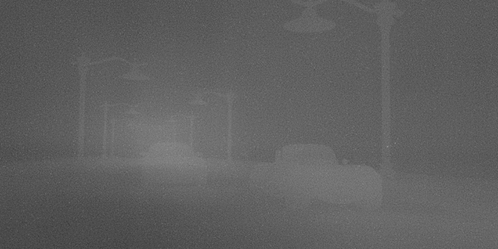
Cars

The beam radiance estimate (left) finds all photons along camera rays, which is a performance bottleneck for the Cars scene due to high volumetric depth complexity and many photons (917K). Our method (right) fits a hierarchical, anisotropic Gaussian mixture model to the photons and can render this scene over two-times faster, and with higher quality, using only (4K) Gaussian components. The listed times denote the costs of the preprocessing stage (including photon tracing and hierarchy construction), as well as the final rendering stage, respectively

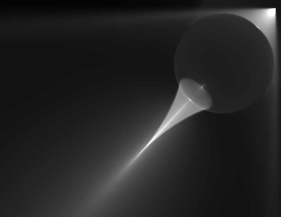
Sphere Caustic

The Sphere Caustic scene comparing the BRE with 2M photons to our 16K-term Gaussian fit.

Museum

In the Museum scene, the high volumetric depth complexity and large number of photons (3.6M) makes the BRE (left) inefficient. Our method addresses these problems by using a hierarchical, anisotropic Gaussian mixture with only 16K Gaussian components.

Ocean

The Ocean scene comparing the BRE with 2M photons to our 16K-term Gaussian fit.

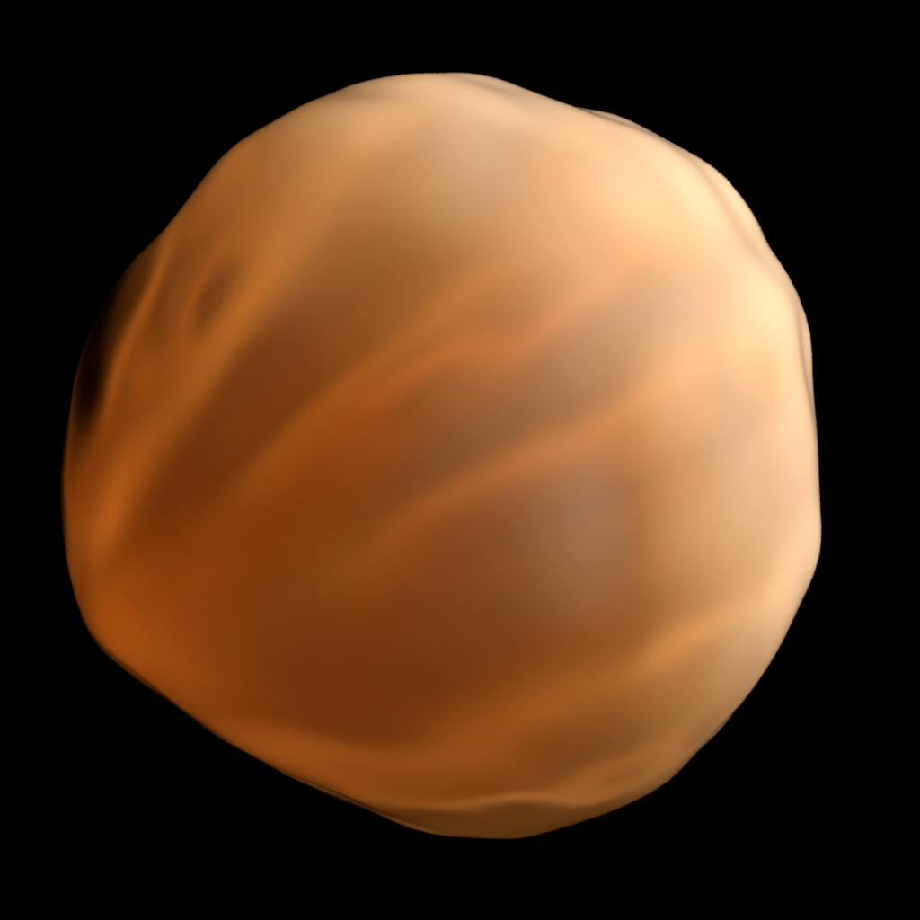
Bumpy Sphere

Renderings of the Bumpy Sphere comparing our method to the corresponding BRE renderings using all photons in the Gaussian fit. The listed times correspond to the preprocessing and rendering stages, respectively.