Introduction
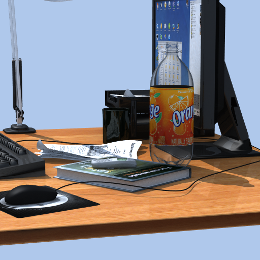
For the final project my goal was to render a realistic cluttered desk scene. I wanted to work on a scene that had lots of texture detail, and that would benefit from some nice global illumination.
Throughout the quarter I have been primarily concerned with quality of the software design, and less concerned with actual quantity of features. I have re-implemented a ray tracer many times and this time I really wanted my design to last and evolve with me. Therefore, I have not yet re-implemented more advanced features such as photon mapping, but feel that for my chosen scene this was not a crucial component.
Features
I did not use Miro as a code base for my renderer; in fact, I haven't actually touched the Miro code since assignment 1. My renderer, affectionately referred to as renderBitch, was essentially written from scratch. I implemented my own lexer and parser using flex and bison for reading in scene description files. renderBitch also has an analogous C++ API which has a structure symmetric to that of the scene file language. It supports loading of various image file formats (PNG, JPEG, Radiance, OpenEXR, TIFF), and supports reading of Wavefront OBJ files with material names and automatic normal smoothing (these two turned out to be an essential features for working on this scene). In addition, I have currently implemented the following geometric primitives:
- Triangles
- Spheres, Cylinders, Cones, Paraboloids, and general Quadrics
- Torus
- Squares, Disks, and Cubes
- Bilinear Patches (not triangulated)
- Bicubic Bezier Patches (not triangulated)
- Curves (for hair)
- Hierarchical grids, Octrees, and BVHs
However, for this scene, only triangles were actually rendered. In addition, I implemented the following features for this project:
- Path tracing
- Irradiance Caching with irradiance gradients
- Texture mapping (both raster and procedural textures)
- Distribution ray tracing (anti-aliasing, depth-of-field, area lights) using QMC and MC sampling
- Fresnel reflection and refraction
- Adaptive trace depth using ray importance and Russian roulette
Irradiance Caching
From the beginning, a major component for my project has been nice diffuse interreflections. For this I implemented irradiance caching with gradients. Using irradiance caching can significantly reduce high frequency noise when compared to path tracing (though at low quality, you trade that for low frequency noise).
Lessons learned
One drawback with the naive irradiance caching algorithm is that it actually tends to work very poorly in common sky-dome renderings. This is due to the way that irradiance caching estimates the valid radius of each irradiance sample. This is done by taking the harmonic mean of the ray distances used to evaluate the sample. The problem arises when all samples hit only the backgrounds: their harmonic mean distance is infinity. This creates an infinite valid radius. In a sky-dome rendering of a single object, it can be very likely that an irradiance evaluation near the horizon does not hit anything but the background. This sample would then result in an infinite valid radius, and no further samples would be generated on the ground plane.
Another, somewhat symmetric problem, is that the regular split-sphere model creates very high concentrations of samples within corners and crevices. This is, for the most part, a desirable feature, since irradiance changes more quickly near corners. However, within a simple Cornel box scene, samples would be placed at essentially every pixel near the edges of the walls. This can be fairly time consuming.
To remedy these two problems, I implemented a minimum and maximum evaluation spacing option. These two options essentially examine each irradiance sample, and after it is computed, clamp the valid radius to be within the desired range. This feature seems to be present in Lightwave's global illumination implementation as well. This addition worked well for closed scenes with limited spatial extent, but since the clamping values are essentially world space units, it does not limit the number of evaluations at the horizon. A pixel-space technique seems appropriate for this situation. I had considered using ray differentials for this task (and later Henrik informed me that that is the way he would approach the problem as well), though it was not essential for my scene, so I have left this for future work.
From the appearance of rendered images, I deduced a while back that Lightwave's "radiosity" is actually irradiance caching (though, seemingly without gradients). Therefore, I planned on using Lightwave's results as a reference when testing my global illumination implementation. For this end, I set up a simple sky-dome scene with the dragon from Stanford. I set the rendering settings identical in both Lightwave and renderBitch (GI tolerance, samples per evaluation, etc) and after some bug hunting, attained the following two results:
 renderBitch
 Lightwave
I also test-rendered a few other models I had created in the past:
Modeling & Texturing
The nature of my scene required me to also do some extensive modeling. I modeled all objects in the scene from scratch using Lightwave, a tape measure, my digital camera, and my physical desk scene (with the exception of the keyboard, which I modified from a keyboard model that comes with Lightwave). Most of the modeling was done using subdivision surfaces - these were then exported as triangle meshes in OBJ format. In addition, I created all the textures using a combination of my digital camera and Photoshop (exception being the wood texture on the desk). I originally planned to at least implementing a nice wood plank texture procedurally, but this idea was abandoned due to time constraints. The final scene contained over X triangles.
Because of the large amount of models and materials in my scene, it was important that I be able to set material properties on more than just a mesh basis. To accomplish this, I used the "usemtl" tag available in OBJ files. Lightwave already had an exporter which wrote out these tags. My scene file parser simply stores the names of the material specified for each polygon in the OBJ file, and if a renderBitch material had been previously defined with the same name, those polygons use that material for shading. So in essence, I can retrieve material groups, but the actual materials themselves are not converted. Also, I had to implement automatic normal smoothing of the OBJ files because Lightwave does not export OBJ files with vertex normals (and my trial version of Deep Exploration ran out :-).
Super-Sampling & Quasi-Monte Carlo
Before I started working on this assignment, I had already implemented simple anti-aliasing using N-Rooks sampling. I chose this technique because, as opposed to jittered sampling, specifying quality using the square root of the number of samples was not required. I was toying with the idea of implementing something more advanced, possibly using quasi-random sampling. I had always wanted to directly visualize my various sampling methods in order to evaluate their distribution quality at a more low-level. Then Steve Rotenberg showed me a little demo which did exactly what I had been planning to do. I was impressed with the usefulness of the demo and it motivated me to create my own. I therefore decided to implement a few quasi-random sequences as well as more traditional sampling methods such as jittered and random sampling. Numerical Recipes was an invaluable resource for this task. I implemented their Sobol sequence generator. In the end, my list of sampling methods included:
- Random sampling
- Jittered Sampling
- Multi-jittered sampling
- N-Rooks (Latin Hypercube) sampling
- Sobol sequence sampling
- Halton sequence sampling
- Hammersley sequence sampling
I was rather surprised by my results. I had always thought that N-Rooks was a fairly good method of distributing samples, but by examining my visualized samples, I quickly discovered that it was nearly as bad as random sampling. This further motivated me to replace N-Rooks sampling with something more advanced.
I ended up using a Hammersley sequence to sample the image and eye. This sequence proved to be the most well distributed of all the techniques I visualized. The only drawback of the Hammersley sequence is that it is not hierarchical. A hierarchical sequence is one which has the property that if you generate n points and separately generate n+1 points, the first n points will be the same in both sets. This allows for incremental sampling. However, I knew ahead of time how many samples I would take per pixel, so this did not cause a problem.
In addition, I added a random offset to the generated Hammersley points in order to eliminate correlation between pixels. Later, I also shuffled the sample points to eliminate any correlation between the image and eye sample points for depth-of-field.
Adaptive Sampling, Soft Shadows & DOF
Naive super-sampling where render time was linearly proportional to the level of anti-aliasing soon proved to be unmanageable. Therefore, I decided relatively early to implement a simple form of adaptive sampling. My scheme first renders the image using 1 sample per pixel. Then, if super-sampling is specified, a threshold image is computed based on a user-provided threshold value. This threshold image is computed by comparing the contrast between neighboring pixels against the threshold value, and is evaluated independently for each color channel:
contrast = |pixelx,y-pixelx-i,y-j|/(pixelx,y+pixelx-i,y-j)
where i and j loop over the local neighborhood of each pixel.
In order to not introduce bias during this process, if a pixel is determined to be super-sampled, the previously computed value is thrown out. Any pixel above the threshold is then super-sampled using a user-specified amount of samples. This scheme proved to be an immense time saver. It allowed me to super sample images with up 10 samples per pixel with only about double the render time.
Having nicely distributed sequences, I was in a perfect position to implement more distribution ray tracing elements, such as soft shadows. The final rendered scene uses a small spherical distant light for the sun. Sampling the light is accomplished by transforming the samples from a unit square into a circular sector of a sphere defined by a maximum angle. This angle is determined using the maximum subtended angle from the point of evaluation towards the area light. The spherical disk is then oriented towards the light and shadow rays are directed towards the sample points. In order to achieve some form of adaptive sampling, the user specifies the minimum number of samples per light. After these are taken, if the samples were either all in shadow or all illuminated, then shadow computation stops; otherwise, more samples are taken to refine the solution. This solution is inherently incremental; so for lights, I use a randomly-shifted Halton sequence since it allows for incremental sampling.
Depth-of-field was implemented using the standard method of generating random samples within a disk representing the eye. For this I needed to transform samples in the unit square into samples in the unit disk. I implemented two methods (polar map, and concentric map) for this and evaluated their distribution characteristics. The concentric map proved to be better distributed, especially if using the same number of samples in both dimensions. To achieve optimal results with the polar map, it was necessary to stratify with 2 or 3 times as many samples in the angular dimension as the radial dimension. For this reason, the concentric map method was used. As mentioned before, the eye and camera samples were shuffled before pairing in order to eliminate correlation.
Adaptive Trace Depth & Russian Roulette
Once I started rendering something resembling my final scene, I ran into the odd fact that enabling both reflection and refraction on a model made the render time explode (much more than the combination of having just reflection and just refraction on). I quickly figured out that this is due to the exponential ray growth when tracing both a reflection and refraction ray at each hit point. I therefore implemented importance for rays, sometimes referred to as ray weights. This importance value is the maximum possible contribution to the rendered image: it starts at 1.0 for eye rays. Assuming physically plausible materials, the importance of a ray diminishes with each bounce.
For my glass and 2-liter bottle, I implemented Fresnel reflections and refractions. Adaptive depth control is used by checking if the importance of the incoming ray is above a certain threshold. If it is, then both a reflection and refraction ray are sent. If it is below the threshold, then Russian roulette is used to shoot only one ray.
Ray importance is also utilized for global illumination and soft shadows. The number of samples for soft shadows is first multiplied by the importance of the ray (and is clamped to be at least 1). This significantly reduces render time when irradiance caching is turned on because secondary diffuse rays do not evaluate precise soft shadow as visually important rays do. Rays shot out during irradiance evaluation each get 1/N of the ray's importance, where N is the number of rays in the evaluation. I had considered using a similar technique to simplify irradiance estimates for unimportant rays, but this is probably undesirable: Certain points in the scene are visible from multiple ray paths. If the point is first encountered using a path which has many specular bounces, this would produce low importance, and a low quality evaluation. However, that same cached evaluation might later be used for a high-importance path.
Work in Progress
Here are some renders I took while building up to the final render during various stages of completeness: