Abstract Data Types (ADTs)
There are two key aspects of any program: what to operate on (the data), and how to operate on it (the functions). Now it's time to think more about the interplay between data and functions.
One powerful approach to dealing with the function-data relationship is to use Abstract Data Types (ADTs), in which we know at a high level what the data represent (but not how it is stored), and more importantly the operations on the data. (Usually the same operations work on a wide class of data types, so these should probably be called "abstract operation types", but it's too late to change the name now.) The idea is to hide the way that the data are represented. Before a paper by Parnas in the 70's, everyone assumed that the natural thing to do was for every function to know how the data were represented and to work with that representation. That's dangerous, since if we ever change the representation, then we have to go change every function that makes use of that representation.
With an ADT, we can perform certain operations supported by an interface, but we can't directly get at the implementation by which the data are represented and the operations supported. It's like an office with a window where a clerk sits and handles your requests to save or retrieve documents. You can't tell if the documents are saved in file cabinets, are scanned into a computer database, etc. There can be multiple implementations of the same ADT where each implementation implements the same functionality, but might use different data structures or algorithms to accomplish the required functionality. You can also change the implementation without affecting any code that only uses the interface.
So today we'll set up an ADT for representing lists. Java provides two List implementations, but soon we'll build up our own. Today we will start with a definition of what a List is and can do (the ADT), and then how an implementation can do that. In fact, over the next few classes we'll implement the list ADT in two very different ways, making efficiency trade-offs but supporting the same uses.
- Defining an ADT: inheritance vs. interface
- The List ADT
- Generics: what does it hold
- Orders of growth
- Asymptotic notation
- Java notes
All the code files for today: SimpleList.java; ArrayListDemo.java; StudentTrackerAppList.java
Defining an ADT: inheritance vs. interfaces
We explored inheritance with Students, and have also used it in a number of other classes, e.g., GUI stuff. Recall that inheritance is used to say that a new subclass "is-a" superclass, plus more stuff / with more specific behaviors. Inheritance captures similarities among classes, in that we can use a subclass in any context where we can use its superclass (but not the other way around). It also propagates implementation details, as the subclass includes the instance variables and associated methods of the superclass.
A related, but different, way to capture similarities is with an
So why would we ever want an interface instead of inheritance? Inheritance can lead to some tricky and ambiguous scenarios. This is particularly true if a class inherits from multiple superclasses, which happen to have different instance variables with the same name or different implementations of a method with the same name. Which one is meant when? (especially if they're called from other objects.) For that reason, Java forbids multiple inheritance; a class can only extend one superclass. It can, however, implement multiple interfaces. There's no ambiguity there — the class provides its own implementation of each method, and doesn't rely on existing (potentially conflicting) implementations that it inherits.
As we saw with inheritance, we can declare a variable to be of the interface type, and not worry about which concrete implementation it is. An example using the List interface: ArrayListDemo.java. Note: you cannot "new" an interface, since it doesn't actually implement anything. You can only "new" a class that implements that interface.
The List ADT
Lists are used to store multiple items of a particular data type. With a List we refer to items by their index. The first item is at index 0, and the last item is at index size-1 (where size is the number of items in the List). Lists in Java are similar to Lists in Python. The closest analog in C is an array.
Unlike an array (in C or in Java), however, Lists do not specify the number of items they hold, and they can grow as items are added. For example, previously we might have declared an array to hold say 10 Student objects. If we needed to track an 11th student, we were out of luck — there was no more memory for the 11th student. With a List, we can easily add the 11th student. We will see how soon.
Our SimpleList interface specifies that the following methods must be implemented:
public int size();returns the number of items in the Listpublic boolean isEmpty();returns true if the List is empty, false otherwisepublic void add(int idx, T item) throws Exception;adds item at index idxpublic void add(T item) throws Exception;adds item at the end of the Listpublic T remove(int idx) throws Exception;removes and returns the item at index idxpublic T get(int idx) throws Exception;returns the item at index idxpublic void set(int idx, T item) throws Exception;replaces the item at index idx with item
Notice that we don't care about what kind of data the List holds. Using get(idx) returns the item at index idx. The functionality does not change according what type of data the List holds. In Java, however, all items in the List must be of the same data type (in Python each List item can have a different data type). But, because an item of a subclass "is a" item of the base class, a List can hold objects declared as a subclass. See Generics below.
We will discuss throws Exception next lecture, but the short answer is that if something goes wrong, the List code can tell the caller that something went wrong, and the caller can decide how to handle it.
Finally, Java provides two implementation of the List ADT for us (note that Java's interface is more complex than our simple interface). The first is called an ArrayList which implements the required List functionality using an array to store data (growing the array if it fills). The second is called a LinkedList which implements the required List functionality using a linked list. Each implementation provides the same ADT functionality, but carry out the operations differently.
Generics: what does it hold
Our interface is generic. We've seen this on the user side with ArrayList, which could hold different things in different cases. So we'd declare, say, ArrayList<Student>. Now on the implementer side, when creating our own generic class/interface, we use a type variable that will consistently hold the type that gets instantiated.
public interface SimpleList<T> {
  ...
  public T get(int index) throws Exception;
  public void add(int idx, T item) throws Exception;
}
Here we have no idea what type of thing will go into our List, and don't really care, so we use the type variable T to stand for whatever someone might use. Thus if someone declares SimpleList<Student>, then T means Student, while for SimpleList<Integer> it means Integer. Just like any variable, it stands for something else, the somewhat odd thing is that the something else is a data type. Typically we name type variables with a single uppercase letter, often T for "type", but sometimes E for "element", or as we'll see later K and V for "key" and "value", and V and E for "vertex" and "edge".
In the body of the code, that type variable consistently means the same thing, which is what gives us type safety. So for SimpleList<Double>, T is always Double, meaning that's the only type we can add to the List, so we can count on exactly what we can do with the stuff in the List.
Orders of growth
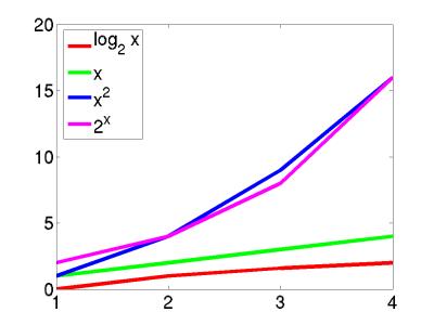
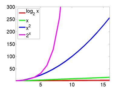
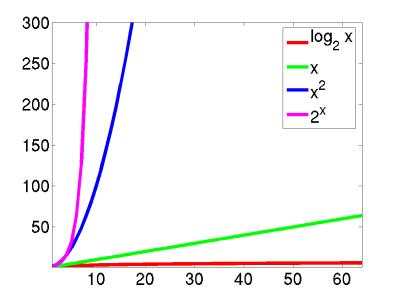
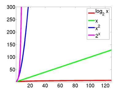
Let's consider the following algorithms on an List containing n items. (I'm assuming you're familiar with these algorithms; give a yell if not.)
- Returning the first element takes an amount of time that is independent of n ("constant time")
- Binary search runs in time proportional to log(n)
- Sequential search runs in time proportional to n
- Many sorting algorithms (such as selection sort) run in time proportional to n². So does any algorithm that deals with all the pairs of numbers runs in time proportional to n² (think of a round-robin tournament).
For example, given {1, 2, 3, 4, 5}, compute:
There are n rows and n columns, so n*n entries.1+1 2+1 ... 5+1 1+2 2+2 ... 5+2 1+3 2+3 ... 5+3 1+4 2+4 ... 5+4 1+5 2+5 ... 5+5 - Algorithms that deal with all possible combinations of the items
run in time 2n.
For example, given {1, 2, 3, 4, 5}, compute:- 1, 2, 3, 4, 5
- 1+2, 1+3, 1+4, 1+5, 2+3, 2+4, 2+5, 3+4, 3+5, 4+5
- 1+2+3, 1+2+4, 1+2+5, 1+3+4, 1+3+5, ...
- 1+2+3+4, ...
- 1+2+3+4+5, ...
Now, computers are always getting faster, but these "orders of growth" help us see at a glance the inherent differences in run-time for different algorithms.
Clearly, when designing algorithms we need to be careful. For example, a brute-force chess algorithm has runtime 2n which makes it completely impractical. Interestingly, though, this type of complexity can help us. In particular, the reason that it is difficult for someone to crack your password is because the best known algorithm for cracking passwords runs in 2n time (specifically factoring large numbers into primes).
Asymptotic notation
So if we're willing to characterize an overall "order of growth", as above, we can get a handle on the major differences. This notion of "grows like" is the essence of the running time — linear search's running time "grows like" n and binary search's running time "grows like" log(n). Computer scientists use it so frequently that we have a special notation for it: "big-Oh" notation, which we write as "O-notation."
For example, the running time of linear search is always at most some linear function of the input size n. Ignoring the coefficients and low-order terms, we write that the running time of linear search is O(n). You can read the O-notation as "order." In other words, O(n) is read as "order n." You'll also hear it spoken as "big-Oh of n" or even just "Oh of n."
Similarly, the running time of binary search is always at most some logarithmic function of the input size n. Again ignoring the coefficients and low-order terms, we write that the running time of binary search is O(lg n), which we would say as "order log n," "big-Oh of log n," or "Oh of log n."
In fact, within our O-notation, if the base of a logarithm is a constant (like 2), then it doesn't really matter. That's because of the formula
loga n = (logb n) / (logb a)for all positive real numbers a, b, and c. In other words, if we compare loga n and logb n, they differ by a factor of logb a, and this factor is a constant if a and b are constants. Therefore, even though we use the "lg" notation within O-notation, it's irrelevant that we're really using base-2 logarithms.
O-notation is used for what we call "asymptotic upper bounds." By "asymptotic" we mean "as the argument (n) gets large." By "upper bound" we mean that O-notation gives us a bound from above on how high the rate of growth is.
Here's the technical definition of O-notation, which will underscore both the "asymptotic" and "upper-bound" notions:
A running time is O(n) if there exist positive constants n0 and c such that for all problem sizes n ≥ n0, the running time for a problem of size n is at most cn.
Here's a helpful picture:
The "asymptotic" part comes from our requirement that we care only about what happens at or to the right of n0, i.e., when n is large. The "upper bound" part comes from the running time being at most cn. The running time can be less than cn, and it can even be a lot less. What we require is that there exists some constant c such that for sufficiently large n, the running time is bounded from above by cn.
For an arbitrary function f(n), which is not necessarily linear, we extend our technical definition:
A running time is O(f(n)) if there exist positive constants n0 and c such that for all problem sizes n ≥ n0, the running time for a problem of size n is at most c f(n).
A picture:

Now we require that there exist some constant c such that for sufficiently large n, the running time is bounded from above by c f(n).
Actually, O-notation applies to functions, not just to running times. But since our running times will be expressed as functions of the input size n, we can express running times using O-notation.
In general, we want as slow a rate of growth as possible, since if the running time grows slowly, that means that the algorithm is relatively fast for larger problem sizes.
We usually focus on the worst case running time, for several reasons:
- The worst case time gives us an upper bound on the time required for any input.
- It gives a guarantee that the algorithm never takes any longer.
- We don't need to make an educated guess and hope that the running time never gets much worse.
You might think that it would make sense to focus on the "average case" rather than the worst case, which is exceptional. And sometimes we do focus on the average case. But often it makes little sense. First, you have to determine just what is the average case for the problem at hand. Suppose we're searching. In some situations, you find what you're looking for early. For example, a video database will put the titles most often viewed where a search will find them quickly. In some situations, you find what you're looking for on average halfway through all the data…for example, a linear search with all search values equally likely. In some situations, you usually don't find what you're looking for.
It is also often true that the average case is about as bad as the worst case. Because the worst case is usually easier to identify than the average case, we focus on the worst case.
Computer scientists use notations analogous to O-notation for "asymptotic lower bounds" (i.e., the running time grows at least this fast) and "asymptotically tight bounds" (i.e., the running time is within a constant factor of some function). We use Ω-notation (that's the Greek leter "omega") to say that the function grows "at least this fast". It is almost the same as Big-O notation, except that is has an "at least" instead of an "at most":
A running time is Ω(n) if there exist positive constants n0 and c such that for all problem sizes n ≥ n0, the running time for a problem of size n is at least cn.
We use Θ-notation (that's the Greek letter "theta") for asymptotically tight bounds:
A running time is Θ(f(n)) if there exist positive constants n0, c1, and c2 such that for all problem sizes n ≥ n0, the running time for a problem of size n is at least c1 f(n) and at most c2 f(n).
Pictorially,
In other words, with Θ-notation, for sufficiently large problem sizes, we have nailed the running time to within a constant factor. As with O-notation, we can ignore low-order terms and constant coefficients in Θ-notation.
Note that Θ-notation subsumes O-notation in that
If a running time is Θ(f(n)), then it is also O(f(n)).
The converse (O(f(n)) implies Θ(f(n))) does not necessarily hold.
The general term that we use for either O-notation or Θ-notation is asymptotic notation.
Recap
Both asymptotic notations—O-notation and Θ-notation—provide ways to characterize the rate of growth of a function f(n). For our purposes, the function f(n) describes the running time of an algorithm, but it really could be any old function. Asymptotic notation describes what happens as n gets large; we don't care about small values of n. We use O-notation to bound the rate of growth from above to within a constant factor, and we use Θ-notation to bound the rate of growth to within constant factors from both above and below.
We need to understand when we can apply each asymptotic notation. For example, in the worst case, linear search runs in time proportional to the input size n; we can say that linear search's worst-case running time is Θ(n). It would also be correct, but less precise, to say that linear search's worst-case running time is O(n). Because in the best case, linear search finds what it's looking for in the first array position it checks, we cannot say that linear search's running time is Θ(n) in all cases. But we can say that linear search's running time is O(n) in all cases, since it never takes longer than some constant times the input size n.
Working with asymptotic notation
Although the definitions of O-notation and Θ-notation may seem a bit daunting, these notations actually make our lives easier in practice. There are two ways in which they simplify our lives:
- Constant factors don't matter
- Constant multiplicative factors are "absorbed" by the multiplicative constants in O-notation (c) and Θ-notation (c1 and c2). For example, the function 1000n2 is Θ(n2), since we can choose both c1 and c2 to be 1000. Although we may care about constant multiplicative factors in practice, we focus on the rate of growth when we analyze algorithms, and the constant factors don't matter. Asymptotic notation is a great way to suppress constant factors.
- Low-order terms don't matter
- When we add or subtract low-order terms, they disappear when using asymptotic notation. For example, consider the function n2 + 1000n. I claim that this function is Θ(n2). Clearly, if I choose c1 = 1, then I have n2 + 1000n ≥ c1n2, so this side of the inequality is taken care of.
The other side is a bit tougher. I need to find a constant c2 such that for sufficiently large n, I'll get that n2 + 1000n ≤ c2n2. Subtracting n2 from both sides gives 1000n ≤ c2n2 – n2 = (c2 – 1) n2. Dividing both sides by (c2 – 1) n gives 1000 / (c2 – 1) ≤ n. Now I have some flexibility, which I'll use as follows. I pick c2 = 2, so that the inequality becomes 1000 / (2 – 1) ≤ n, or 1000 ≤ n. Now I'm in good shape, because I have shown that if I choose n0 = 1000 and c2 = 2, then for all n ≥ n0, I have 1000 ≤ n, which we saw is equivalent to n2 + 1000n ≤ c2n2.
The point of this example is to show that adding or subtracting low-order terms just changes the n0 that we use. In our practical use of asymptotic notation, we can just drop low-order terms.
In combination, constant factors and low-order terms don't matter. If we see a function like 1000n2 – 200n, we can ignore the low-order term 200n and the constant factor 1000, and therefore we can say that 1000n2 – 200n is Θ(n2).
As we have seen, we use O-notation for asymptotic upper bounds and Θ-notation for asymptotically tight bounds. Θ-notation is more precise than O-notation. Therefore, we prefer to use Θ-notation whenever it's appropriate to do so. We shall see times, however, in which we cannot say that a running time is tight to within a constant factor both above and below. Sometimes, we can only bound a running time from above. In other words, we might only be able to say that the running time is no worse than a certain function of n, but it might be better. In such cases, we'll have to use O-notation, which is perfect for such situations.
Java notes
- data structure
- A concrete way to store data in the computer. For example, an array or linked list.
- Abstract Data Type (ADT)
- Defines a set of operations to be performed on a collection of data. Note that: An ADT does not specify the type of data it operates on. In fact, it should operate the same way on any type of data (such as Strings, integers, or Objects). An ADT does not specify the type of data structure used to store elements (such as an array or linked list). That is left up to the implementation. Lists are an example of an ADT. We will soon implement other ADTs such as Set and Maps.
- interface
- A file that specifies a set of method signatures that must be implemented. An interface is how Java learns about the ADT operations that must be carried out for an ADT. An interface does not define instance variables and does not provide implementations for those methods. When a class "implements" an interface, it must provide implementations for every method signature in the interface. Note that: interfaces are actual .java files that you create, unlike ADTs which are a just description of operations and what each one does. Examples of an interface include our SimpleList.java which is a simplified version of Java's built-in List interface. We will implement our SimpleList interface with a linked link in SinglyLinked.java and we will write a separate implementation using an array with GrowingArray.java. Each implementation carries out the List ADT methods declared in the interface, but does so storing data in a different data structure (e.g., in a linked list or in an array). Similarly, the designers of Java implemented the List ADT with a linked list in LinkedList and also with an array in ArrayList. We will write our own implementations to see what the designers of Java did when they implemented LinkedList and ArrayList.